18. Non-Conjugate Priors#

GPU

This lecture was built using a machine with the latest CUDA and CUDANN frameworks installed with access to a GPU.

To run this lecture on Google Colab, click on the “play” icon top right, select Colab, and set the runtime environment to include a GPU.

To run this lecture on your own machine, you need to install the software listed following this notice.

!pip install numpyro jax

This lecture is a sequel to the Two Meanings of Probability.

That lecture offers a Bayesian interpretation of probability in a setting in which the likelihood function and the prior distribution over parameters just happened to form a conjugate pair in which

application of Bayes’ Law produces a posterior distribution that has the same functional form as the prior

Having a likelihood and prior that are conjugate can simplify calculation of a posterior, facilitating analytical or nearly analytical calculations.

But in many situations the likelihood and prior need not form a conjugate pair.

after all, a person’s prior is his or her own business and would take a form conjugate to a likelihood only by remote coincidence

In these situations, computing a posterior can become very challenging.

In this lecture, we illustrate how modern Bayesians confront non-conjugate priors by using Monte Carlo techniques that involve

first cleverly forming a Markov chain whose invariant distribution is the posterior distribution we want
simulating the Markov chain until it has converged and then sampling from the invariant distribution to approximate the posterior

We shall illustrate the approach by deploying a powerful Python library, NumPyro that implements this approach.

As usual, we begin by importing some Python code.

import numpy as np
import seaborn as sns
import matplotlib.pyplot as plt
import scipy.stats as st

from dataclasses import dataclass, field
from typing import NamedTuple
import jax.numpy as jnp
from jax import random as jax_random

import numpyro
from numpyro import distributions as ndist
import numpyro.distributions.constraints as nconstraints
from numpyro.infer import MCMC as nMCMC
from numpyro.infer import NUTS as nNUTS
from numpyro.infer import SVI as nSVI
from numpyro.infer import Trace_ELBO as nTrace_ELBO
from numpyro.optim import Adam as nAdam

18.1. Unleashing MCMC on a binomial likelihood#

This lecture begins with the binomial example in the Two Meanings of Probability.

That lecture computed a posterior

analytically via choosing the conjugate priors,

This lecture instead computes posteriors

numerically by sampling from the posterior distribution through MCMC methods, and
using a variational inference (VI) approximation.

We use numpyro with assistance from jax to approximate a posterior distribution.

We use several alternative prior distributions.

We compare computed posteriors with ones associated with a conjugate prior as described in Two Meanings of Probability.

18.1.1. Analytical posterior#

Assume that the random variable $X \sim B i n o m (n, θ)$ .

This defines a likelihood function

L (Y | θ) = Prob (X = k | θ) = (\frac{n!}{k! (n - k)!}) θ^{k} (1 - θ)^{n - k}

where $Y = k$ is an observed data point.

We view $θ$ as a random variable for which we assign a prior distribution having density $f (θ)$ .

We will try alternative priors later, but for now, suppose the prior is distributed as $θ \sim B e t a (α, β)$ , i.e.,

f (θ) = Prob (θ) = \frac{θ^{α - 1} (1 - θ)^{β - 1}}{B (α, β)}

We choose this as our prior for now because we know that a conjugate prior for the binomial likelihood function is a beta distribution.

After observing $k$ successes among $N$ sample observations, the posterior probability distribution of $θ$ is

Prob (θ | k) = \frac{Prob (θ, k)}{Prob (k)} = \frac{Prob (k | θ) Prob (θ)}{Prob (k)} = \frac{Prob (k | θ) Prob (θ)}{\int_{0}^{1} Prob (k | θ) Prob (θ) d θ}

= \frac{(\binom{N}{k}) (1 - θ)^{N - k} θ^{k} \frac{θ^{α - 1} (1 - θ)^{β - 1}}{B (α, β)}}{\int_{0}^{1} (\binom{N}{k}) (1 - θ)^{N - k} θ^{k} \frac{θ^{α - 1} (1 - θ)^{β - 1}}{B (α, β)} d θ}

= \frac{(1 - θ)^{β + N - k - 1} θ^{α + k - 1}}{\int_{0}^{1} (1 - θ)^{β + N - k - 1} θ^{α + k - 1} d θ} .

Thus,

Prob (θ | k) \sim B e t a (α + k, β + N - k)

The analytical posterior for a given conjugate beta prior is coded in the following

def simulate_draw(theta, n):
    """Draws a Bernoulli sample of size n with probability P(Y=1) = theta"""
    rand_draw = np.random.rand(n)
    draw = (rand_draw < theta).astype(int)
    return draw


def analytical_beta_posterior(data, alpha0, beta0):
    """
    Computes analytically the posterior distribution with beta prior parametrized by (alpha, beta)
    given # num observations

    Parameters
    ---------
    num : int.
        the number of observations after which we calculate the posterior
    alpha0, beta0 : float.
        the parameters for the beta distribution as a prior

    Returns
    ---------
    The posterior beta distribution
    """
    num = len(data)
    up_num = data.sum()
    down_num = num - up_num
    return st.beta(alpha0 + up_num, beta0 + down_num)

18.1.2. Two ways to approximate posteriors#

Suppose that we don’t have a conjugate prior.

Then we can’t compute posteriors analytically.

Instead, we use computational tools to approximate the posterior distribution for a set of alternative prior distributions using numpyro.

We first use the Markov Chain Monte Carlo (MCMC) algorithm.

We implement the NUTS sampler to sample from the posterior.

In that way we construct a sampling distribution that approximates the posterior.

After doing that we deploy another procedure called Variational Inference (VI).

In particular, we implement Stochastic Variational Inference (SVI) machinery in numpyro.

The MCMC algorithm supposedly generates a more accurate approximation since in principle it directly samples from the posterior distribution.

But it can be computationally expensive, especially when dimension is large.

A VI approach can be cheaper, but it is likely to produce an inferior approximation to the posterior, for the simple reason that it requires guessing a parametric guide functional form that we use to approximate a posterior.

This guide function is likely at best to be an imperfect approximation.

By paying the cost of restricting the putative posterior to have a restricted functional form, the problem of approximating a posterior is transformed to a well-posed optimization problem that seeks parameters of the putative posterior that minimize a Kullback-Leibler (KL) divergence between true posterior and the putative posterior distribution.

minimizing the KL divergence is equivalent to maximizing a criterion called the Evidence Lower Bound (ELBO), as we shall verify soon.

18.2. Prior distributions#

In order to be able to apply MCMC sampling or VI, numpyro requires that a prior distribution satisfy special properties:

we must be able to sample from it;
we must be able to compute the log pdf pointwise;
the pdf must be differentiable with respect to the parameters.

We’ll want to define a distribution class.

We will use the following priors:

a uniform distribution on $[\underset{―}{θ}, \overset{―}{θ}]$ , where $0 \leq \underset{―}{θ} < \overset{―}{θ} \leq 1$ .
a truncated log-normal distribution with support on $[0, 1]$ with parameters $(μ, σ)$ .
- To implement this, let $Z \sim N o r m a l (μ, σ)$ and $\tilde{Z}$ be truncated normal with support $[- \infty, \log (1)]$ , then $\exp (Z)$ has a log normal distribution with bounded support $[0, 1]$ . This can be easily coded since numpyro has a built-in truncated normal distribution, and numpyro’s TransformedDistribution class that includes an exponential transformation.
a shifted von Mises distribution that has support confined to $[0, 1]$ with parameter $(μ, κ)$ .
- Let $X \sim v o n M i s e s (0, κ)$ . We know that $X$ has bounded support $[- π, π]$ . We can define a shifted von Mises random variable $\tilde{X} = a + b X$ where $a = 0.5, b = 1 / (2 π)$ so that $\tilde{X}$ is supported on $[0, 1]$ .
- This can be implemented using numpyro’s TransformedDistribution class with its AffineTransform method.
a truncated Laplace distribution.
- We also considered a truncated Laplace distribution because its density comes in a piece-wise non-smooth form and has a distinctive spiked shape.
- The truncated Laplace can be created using numpyro’s TruncatedDistribution class.

def TruncatedLogNormal_trans(loc, scale):
    """
    Obtains the truncated log normal distribution using numpyro's TruncatedNormal and ExpTransform
    """
    base_dist = ndist.TruncatedNormal(
        low=-jnp.inf, high=jnp.log(1), loc=loc, scale=scale
    )
    return ndist.TransformedDistribution(base_dist, ndist.transforms.ExpTransform())


def ShiftedVonMises(kappa):
    """Obtains the shifted von Mises distribution using AffineTransform"""
    base_dist = ndist.VonMises(0, kappa)
    return ndist.TransformedDistribution(
        base_dist, ndist.transforms.AffineTransform(loc=0.5, scale=1 / (2 * jnp.pi))
    )


def TruncatedLaplace(loc, scale):
    """Obtains the truncated Laplace distribution on [0,1]"""
    base_dist = ndist.Laplace(loc, scale)
    return ndist.TruncatedDistribution(base_dist, low=0.0, high=1.0)

18.2.1. Variational inference#

Instead of directly sampling from the posterior, the variational inference method approximates an unknown posterior distribution with a family of tractable distributions/densities.

It then seeks to minimize a measure of statistical discrepancy between the approximating and true posteriors.

Thus variational inference (VI) approximates a posterior by solving a minimization problem.

Let the latent parameter/variable that we want to infer be $θ$ .

Let the prior be $p (θ)$ and the likelihood be $p (Y | θ)$ .

We want $p (θ | Y)$ .

Bayes’ rule implies

p (θ | Y) = \frac{p (Y, θ)}{p (Y)} = \frac{p (Y | θ) p (θ)}{p (Y)}

where

(18.1)#

p (Y) = \int p (Y ∣ θ) p (Y) d θ .

The integral on the right side of (18.1) is typically difficult to compute.

Consider a guide distribution $q_{ϕ} (θ)$ parameterized by $ϕ$ that we’ll use to approximate the posterior.

We choose parameters $ϕ$ of the guide distribution to minimize a Kullback-Leibler (KL) divergence between the approximate posterior $q_{ϕ} (θ)$ and the posterior:

D_{K L} (q (θ; ϕ) ‖ p (θ ∣ Y)) \equiv - \int q (θ; ϕ) \log \frac{p (θ ∣ Y)}{q (θ; ϕ)} d θ

Thus, we want a variational distribution $q$ that solves

min_{ϕ} D_{K L} (q (θ; ϕ) ‖ p (θ ∣ Y))

Note that

\begin{array}{r} \begin{aligned} D_{K L} (q (θ; ϕ) ‖ p (θ ∣ Y)) & = - \int q (θ; ϕ) \log \frac{P (θ ∣ Y)}{q (θ; ϕ)} d θ \\ = - \int q (θ) \log \frac{\frac{p (θ, Y)}{p (Y)}}{q (θ)} d θ \\ = - \int q (θ) \log \frac{p (θ, Y)}{p (θ) q (Y)} d θ \\ = - \int q (θ) [\log \frac{p (θ, Y)}{q (θ)} - \log p (Y)] d θ \\ = - \int q (θ) \log \frac{p (θ, Y)}{q (θ)} + \int q (θ) \log p (Y) d θ \\ = - \int q (θ) \log \frac{p (θ, Y)}{q (θ)} d θ + \log p (Y) \\ \log p (Y) & = D_{K L} (q (θ; ϕ) ‖ p (θ ∣ Y)) + \int q_{ϕ} (θ) \log \frac{p (θ, Y)}{q_{ϕ} (θ)} d θ \end{aligned} \end{array}

For observed data $Y$ , $p (θ, Y)$ is a constant, so minimizing KL divergence is equivalent to maximizing

(18.2)#

E L B O \equiv \int q_{ϕ} (θ) \log \frac{p (θ, Y)}{q_{ϕ} (θ)} d θ = E_{q_{ϕ} (θ)} [\log p (θ, Y) - \log q_{ϕ} (θ)]

Formula (18.2) is called the evidence lower bound (ELBO).

A standard optimization routine can be used to search for the optimal $ϕ$ in our parametrized distribution $q_{ϕ} (θ)$ .

The parameterized distribution $q_{ϕ} (θ)$ is called the variational distribution.

We can implement Stochastic Variational Inference (SVI) in numpyro using the Adam gradient descent algorithm to approximate the posterior.

We use two sets of variational distributions: Beta and TruncatedNormal with support $[0, 1]$

Learnable parameters for the Beta distribution are (alpha, beta), both of which are positive.
Learnable parameters for the Truncated Normal distribution are (loc, scale).

Note

We restrict the truncated Normal parameter ‘loc’ to be in the interval $[0, 1]$

18.3. Implementation#

We have constructed a Python class BayesianInference that requires the following arguments to be initialized:

param: a tuple/scalar of parameters dependent on distribution types
name_dist: a string that specifies distribution names

The (param, name_dist) pair includes:

(alpha, beta, ‘beta’)
(lower_bound, upper_bound, ‘uniform’)
(loc, scale, ‘lognormal’)
- Note: This is the truncated log normal.
(kappa, ‘vonMises’), where kappa denotes concentration parameter, and center location is set to $0.5$ . Using numpyro, this is the shifted distribution.
(loc, scale, ‘laplace’)
- Note: This is the truncated Laplace

The class BayesianInference has several key methods :

sample_prior:
- This can be used to draw a single sample from the given prior distribution.
show_prior:
- Plots the approximate prior distribution by repeatedly drawing samples and fitting a kernel density curve.
MCMC_sampling:
- INPUT: (data, num_samples, num_warmup=1000)
- Takes a jnp.array data and generates MCMC sampling of posterior of size num_samples.
SVI_run:
- INPUT: (data, guide_dist, n_steps=10000)
- guide_dist = ‘normal’ - use a truncated normal distribution as the parametrized guide
- guide_dist = ‘beta’ - use a beta distribution as the parametrized guide
- RETURN: (params, losses) - the learned parameters in a dict and the vector of loss at each step.

class BayesianInference(NamedTuple):
    """
    Parameters
    ---------
    param : tuple.
        a tuple object that contains all relevant parameters for the distribution
    dist : str.
        name of the distribution - 'beta', 'uniform', 'lognormal', 'vonMises', 'tent'
    """
    param: tuple
    name_dist: str
    # jax requires explicit PRNG state to be passed
    rng_key: jax_random.PRNGKey = jax_random.PRNGKey(0)


def sample_prior(model: BayesianInference):
    """Define the prior distribution to sample from in numpyro models."""
    if model.name_dist == "beta":
        # unpack parameters
        alpha0, beta0 = model.param
        sample = numpyro.sample(
            "theta", ndist.Beta(alpha0, beta0), rng_key=model.rng_key
        )

    elif model.name_dist == "uniform":
        # unpack parameters
        lb, ub = model.param
        sample = numpyro.sample(
            "theta", ndist.Uniform(lb, ub), rng_key=model.rng_key
        )

    elif model.name_dist == "lognormal":
        # unpack parameters
        loc, scale = model.param
        sample = numpyro.sample(
            "theta", TruncatedLogNormal_trans(loc, scale), rng_key=model.rng_key
        )

    elif model.name_dist == "vonMises":
        # unpack parameters
        kappa = model.param
        sample = numpyro.sample(
            "theta", ShiftedVonMises(kappa), rng_key=model.rng_key
        )

    elif model.name_dist == "laplace":
        # unpack parameters
        loc, scale = model.param
        sample = numpyro.sample(
            "theta", TruncatedLaplace(loc, scale), rng_key=model.rng_key
        )

    return sample


def show_prior(
    model: BayesianInference, size=1e5, bins=20, disp_plot=1
    ):
    """
    Visualizes prior distribution by sampling from prior and plots the approximated sampling distribution
    """
    with numpyro.plate("show_prior", size=size):
        sample = sample_prior(model)
    # to JAX array
    sample_array = jnp.asarray(sample)

    # plot histogram and kernel density
    if disp_plot == 1:
        sns.displot(
            sample_array, kde=True, stat="density", bins=bins, height=5, aspect=1.5
        )
        plt.xlim(0, 1)
        plt.show()
    else:
        return sample_array


def set_model(model: BayesianInference, data):
    """
    Define the probabilistic model by specifying prior, conditional likelihood, and data conditioning
    """
    theta = sample_prior(model)
    output = numpyro.sample(
        "obs", ndist.Binomial(len(data), theta), obs=jnp.sum(data)
    )


def MCMC_sampling(
    model: BayesianInference, data, num_samples, num_warmup=1000
    ):
    """
    Computes numerically the posterior distribution with beta prior parametrized by (alpha0, beta0)
    given data using MCMC
    """
    data = jnp.array(data, dtype=float)
    nuts_kernel = nNUTS(set_model)
    mcmc = nMCMC(
        nuts_kernel,
        num_samples=num_samples,
        num_warmup=num_warmup,
        progress_bar=False,
    )
    mcmc.run(model.rng_key, model=model, data=data)

    samples = mcmc.get_samples()["theta"]
    return samples


# arguments in this function are used to align with the arguments in set_model()
# this is required by svi.run()
def beta_guide(model: BayesianInference, data):
    """
    Defines the candidate parametrized variational distribution that we train to approximate posterior with numpyro
    Here we use parameterized beta
    """
    alpha_q = numpyro.param("alpha_q", 10, constraint=nconstraints.positive)
    beta_q = numpyro.param("beta_q", 10, constraint=nconstraints.positive)

    numpyro.sample("theta", ndist.Beta(alpha_q, beta_q))


# similar with beta_guide()
def truncnormal_guide(model: BayesianInference, data):
    """
    Defines the candidate parametrized variational distribution that we train to approximate posterior with numpyro
    Here we use truncated normal on [0,1]
    """
    loc = numpyro.param("loc", 0.5, constraint=nconstraints.interval(0.0, 1.0))
    scale = numpyro.param("scale", 1, constraint=nconstraints.positive)
    numpyro.sample("theta", ndist.TruncatedNormal(loc, scale, low=0.0, high=1.0))


def SVI_init(model: BayesianInference, guide_dist, lr=0.0005):
    """Initiate SVI training mode with Adam optimizer"""
    adam_params = {"lr": lr}

    if guide_dist == "beta":
        optimizer = nAdam(step_size=lr)
        svi = nSVI(
            set_model, beta_guide, optimizer, loss=nTrace_ELBO()
        )
    elif guide_dist == "normal":
        optimizer = nAdam(step_size=lr)
        svi = nSVI(
            set_model, truncnormal_guide, optimizer, loss=nTrace_ELBO()
        )
    else:
        print("WARNING: Please input either 'beta' or 'normal'")
        svi = None

    return svi


def SVI_run(model: BayesianInference, data, guide_dist, n_steps=10000):
    """
    Runs SVI and returns optimized parameters and losses

    Returns
    --------
    params : the learned parameters for guide
    losses : a vector of loss at each step
    """

    # initiate SVI
    svi = SVI_init(model, guide_dist)

    data = jnp.array(data, dtype=float)
    result = svi.run(
        model.rng_key, n_steps, model, data, progress_bar=False
        )
    params = dict((key, jnp.asarray(value)) for key, value in result.params.items())
    losses = jnp.asarray(result.losses)

    return params, losses

18.4. Alternative prior distributions#

Let’s see how well our sampling algorithm does in approximating

a log normal distribution
a uniform distribution

To examine our alternative prior distributions, we’ll plot approximate prior distributions below by calling the show_prior method.

# truncated log normal
exampleLN = BayesianInference(param=(0, 2), name_dist="lognormal")
show_prior(exampleLN, size=100000, bins=20)

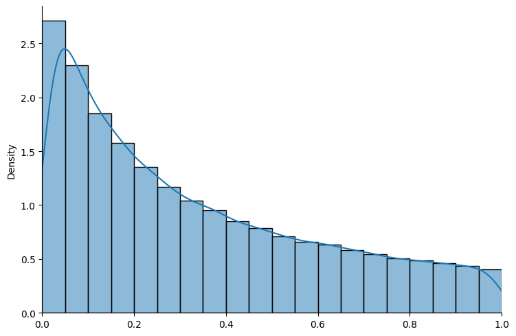
_images/1bea2805ca3c4be8fb08b647d35583121ffecc4fc4df21ebffd093a1d0070da2.png — Fig. 18.1 Truncated log normal distribution#

# truncated uniform
exampleUN = BayesianInference(param=(0.1, 0.8), name_dist="uniform")
show_prior(exampleUN, size=100000, bins=20)

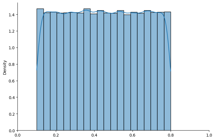
_images/6a1cfca0857599345a533a4e94a2189e0cb12e0c80dae062c24423fed93ceccb.png — Fig. 18.2 Truncated uniform distribution#

The above graphs show that sampling seems to work well with both distributions.

Now let’s see how well things work with von Mises distributions.

# shifted von Mises
exampleVM = BayesianInference(param=10, name_dist="vonMises")
show_prior(exampleVM, size=100000, bins=20)

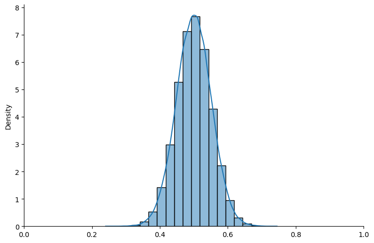
_images/61bb32bf7348463064c150aeb33b8f5f8d9646d434b55dc66292f4802b2b2797.png — Fig. 18.3 Shifted von Mises distribution#

The graphs look good too.

Now let’s try with a Laplace distribution.

# truncated Laplace
exampleLP = BayesianInference(param=(0.5, 0.05), name_dist="laplace")
show_prior(exampleLP, size=100000, bins=20)

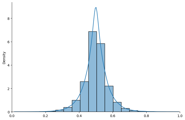
_images/371ef9161eb617ad9383eec7608e5830bb1e4f2574f3305778433e2aa771a831.png — Fig. 18.4 Truncated Laplace distribution#

Having assured ourselves that our sampler seems to do a good job, let’s put it to work in using MCMC to compute posterior probabilities.

18.5. Posteriors via MCMC and VI#

We construct a class BayesianInferencePlot to implement MCMC or VI algorithms and plot multiple posteriors for different updating data sizes and different possible priors.

This class takes as inputs the true data generating parameter theta, a list of updating data sizes for multiple posterior plotting, and a defined and parametrized BayesianInference class.

It has two key methods:

BayesianInferencePlot.MCMC_plot() takes desired MCMC sample size as input and plots the output posteriors together with the prior defined in BayesianInference class.
BayesianInferencePlot.SVI_plot() takes desired VI distribution class (‘beta’ or ‘normal’) as input and plots the posteriors together with the prior.

@dataclass
class BayesianInferencePlot:
    """
    Easily implement the MCMC and VI inference for a given instance of BayesianInference class and
    plot the prior together with multiple posteriors

    Parameters
    ----------
    theta : float.
        the true DGP parameter
    N_list : list.
        a list of sample size
    BayesianInferenceClass : class.
        a class initiated using BayesianInference()

    """

    """Enter Parameters for data generation and plotting"""
    theta: float
    N_list: list
    BayesianInferenceClass: BayesianInference

    # plotting parameters
    binwidth: float = 0.02
    linewidth: float = 0.05
    colorlist: list = field(init=False)

    # data generation
    N_max: float = field(init=False)
    data: np.array = field(init=False)

    def __post_init__(self):
        self.colorlist = sns.color_palette(n_colors=len(self.N_list))
        self.N_max = max(self.N_list)
        self.data = simulate_draw(self.theta, self.N_max)


def MCMC_plot(
    plot_model: BayesianInferencePlot, num_samples, num_warmup=1000
    ):
    fig, ax = plt.subplots()

    # plot prior
    prior_sample = show_prior(
        plot_model.BayesianInferenceClass, disp_plot=0
        )
    sns.histplot(
        data=prior_sample,
        kde=True,
        stat="density",
        binwidth=plot_model.binwidth,
        color="#4C4E52",
        linewidth=plot_model.linewidth,
        alpha=0.1,
        ax=ax,
        label="Prior distribution",
    )

    # plot posteriors
    for id, n in enumerate(plot_model.N_list):
        samples = MCMC_sampling(
            plot_model.BayesianInferenceClass, plot_model.data[:n], num_samples, num_warmup
        )
        sns.histplot(
            samples,
            kde=True,
            stat="density",
            binwidth=plot_model.binwidth,
            linewidth=plot_model.linewidth,
            alpha=0.2,
            color=plot_model.colorlist[id - 1],
            label=f"Posterior with $n={n}$",
        )
    ax.legend(loc="upper left")
    plt.xlim(0, 1)
    plt.show()


def SVI_fitting(guide_dist, params):
    """Fit the beta/truncnormal curve using parameters trained by SVI."""
    # create x axis
    xaxis = jnp.linspace(0, 1, 1000)
    if guide_dist == "beta":
        y = st.beta.pdf(xaxis, a=params["alpha_q"], b=params["beta_q"])

    elif guide_dist == "normal":
        # rescale upper/lower bound. See Scipy's truncnorm doc
        lower, upper = (0, 1)
        loc, scale = params["loc"], params["scale"]
        a, b = (lower - loc) / scale, (upper - loc) / scale

        y = st.truncnorm.pdf(
            xaxis, a=a, b=b, loc=loc, scale=scale
        )
    return (xaxis, y)


def SVI_plot(
    plot_model: BayesianInferencePlot, guide_dist, n_steps=2000
    ):
    fig, ax = plt.subplots()

    # plot prior
    prior_sample = show_prior(plot_model.BayesianInferenceClass, disp_plot=0)
    sns.histplot(
        data=prior_sample,
        kde=True,
        stat="density",
        binwidth=plot_model.binwidth,
        color="#4C4E52",
        linewidth=plot_model.linewidth,
        alpha=0.1,
        ax=ax,
        label="Prior distribution",
    )

    # plot posteriors
    for id, n in enumerate(plot_model.N_list):
        (params, losses) = SVI_run(
            plot_model.BayesianInferenceClass, plot_model.data[:n], guide_dist, n_steps
        )
        x, y = SVI_fitting(guide_dist, params)
        ax.plot(
            x,
            y,
            alpha=1,
            color=plot_model.colorlist[id - 1],
            label=f"Posterior with $n={n}$",
        )
    ax.legend(loc="upper left")
    plt.xlim(0, 1)
    plt.show()

Let’s set some parameters that we’ll use in all of the examples below.

To save computer time at first, notice that we’ll set MCMC_num_samples = 2000 and SVI_num_steps = 5000.

(Later, to increase accuracy of approximations, we’ll want to increase these.)

num_list = [5, 10, 50, 100, 1000]
MCMC_num_samples = 2000
SVI_num_steps = 5000

# theta is the data generating process
true_theta = 0.8

18.5.1. Beta prior and posteriors:#

Let’s compare outcomes when we use a Beta prior.

For the same Beta prior, we shall

compute posteriors analytically
compute posteriors using MCMC using numpyro.
compute posteriors using VI using numpyro.

Let’s start with the analytical method that we described in this Two Meanings of Probability

# first examine Beta prior
BETA = BayesianInference(param=(5, 5), name_dist="beta")

BETA_plot = BayesianInferencePlot(true_theta, num_list, BETA)

# plot analytical Beta prior and posteriors
xaxis = jnp.linspace(0, 1, 1000)
y_prior = st.beta.pdf(xaxis, 5, 5)

fig, ax = plt.subplots()
# plot analytical beta prior
ax.plot(xaxis, y_prior, label="Analytical Beta prior", color="#4C4E52")

data, colorlist, N_list = BETA_plot.data, BETA_plot.colorlist, BETA_plot.N_list

# Plot analytical beta posteriors
for id, n in enumerate(N_list):
    func = analytical_beta_posterior(data[:n], alpha0=5, beta0=5)
    y_posterior = func.pdf(xaxis)
    ax.plot(
        xaxis,
        y_posterior,
        color=colorlist[id - 1],
        label=f"Analytical Beta posterior with $n={n}$",
    )
ax.legend(loc="upper left")
plt.xlim(0, 1)
plt.show()

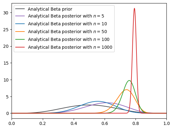
_images/81aab0787c73d6e14a395d4ca6f46495e1df4de63c31a6a933c94ab4f2074efc.png — Fig. 18.5 Analytical density (Beta prior)#

Now let’s use MCMC while still using a beta prior.

We’ll do this for both MCMC and VI.

MCMC_plot(
    BETA_plot, num_samples=MCMC_num_samples
)

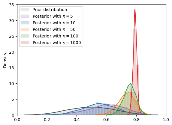
_images/4c8327c04243810c36eb54108e68b0ee410a5409599fa2722e84e29fbcb7f7fe.png — Fig. 18.6 MCMC density (Beta prior)#

SVI_plot(
    BETA_plot, guide_dist="beta", n_steps=SVI_num_steps
)

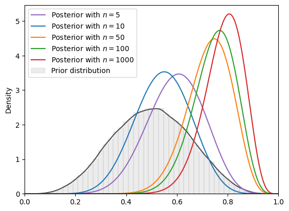
_images/5e87b255e86ab96f03bd8a2cdc204dbb73a81b232f678b4a6b319aab673bb063.png — Fig. 18.7 SVI density (Beta prior, Beta guide)#

Here the MCMC approximation looks good.

But the VI approximation doesn’t look so good.

even though we use the beta distribution as our guide, the VI approximated posterior distributions do not closely resemble the posteriors that we had just computed analytically.

(Here, our initial parameter for Beta guide is (0.5, 0.5).)

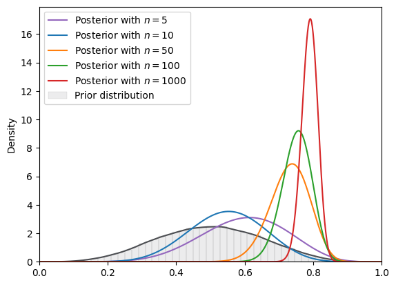
But if we increase the number of steps from 5000 to 100000 in VI as we now shall do, we’ll get VI-approximated posteriors that will be more accurate, as we shall see next.

(Increasing the step size increases computational time though).

SVI_plot(
    BETA_plot, guide_dist="beta", n_steps=100000
)

_images/ce8ab9af5d796db176b0ba94dd60f4fe415a1a6369d2c075030e071a0af1be52.png

18.6. Non-conjugate prior distributions#

Having assured ourselves that our MCMC and VI methods can work well when we have a conjugate prior and so can also compute analytically, we next proceed to situations in which our prior is not a beta distribution, so we don’t have a conjugate prior.

So we will have non-conjugate priors and are cast into situations in which we can’t calculate posteriors analytically.

18.6.1. MCMC#

First, we implement and display MCMC.

We first initialize the BayesianInference classes and then can directly call BayesianInferencePlot to plot both MCMC and SVI approximating posteriors.

# Initialize BayesianInference classes
# Try uniform
STD_UNIFORM = BayesianInference(param=(0, 1), name_dist="uniform")
UNIFORM = BayesianInference(param=(0.2, 0.7), name_dist="uniform")

# Try truncated log normal
LOGNORMAL = BayesianInference(param=(0, 2), name_dist="lognormal")

# Try Von Mises
VONMISES = BayesianInference(param=10, name_dist="vonMises")

# Try Laplace
LAPLACE = BayesianInference(param=(0.5, 0.07), name_dist="laplace")

# Uniform
example_CLASS = STD_UNIFORM
print(
    f"=======INFO=======\nParameters: {example_CLASS.param}\nPrior Dist: {example_CLASS.name_dist}"
)
example_plotCLASS = BayesianInferencePlot(
    true_theta, num_list, example_CLASS
    )
MCMC_plot(
    example_plotCLASS, num_samples=MCMC_num_samples
)

=======INFO=======
Parameters: (0, 1)
Prior Dist: uniform

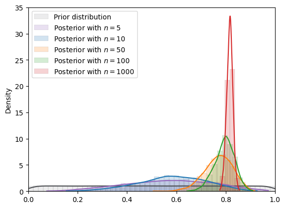
_images/bff06a44b2b0b0cab6fd01abeef5031d715ab74792b545a2b2806bfb33673d1c.png — Fig. 18.8 MCMC density (uniform prior)#

example_CLASS = UNIFORM
print(
    f"=======INFO=======\nParameters: {example_CLASS.param}\nPrior Dist: {example_CLASS.name_dist}"
)
example_plotCLASS = BayesianInferencePlot(
    true_theta, num_list, example_CLASS
    )
MCMC_plot(
    example_plotCLASS, num_samples=MCMC_num_samples
)

=======INFO=======
Parameters: (0.2, 0.7)
Prior Dist: uniform

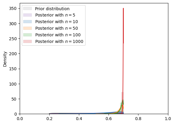
_images/a6409150fefdd1703f64a9ca821f86bea6bd871cfc15357269a3c2d9c9504372.png — Fig. 18.9 MCMC density (uniform prior)#

In the situation depicted above, we have assumed a $U n i f o r m (\underset{―}{θ}, \overset{―}{θ})$ prior that puts zero probability outside a bounded support that excludes the true value.

Consequently, the posterior cannot put positive probability above $\overset{―}{θ}$ or below $\underset{―}{θ}$ .

Note how when the true data-generating $θ$ is located at $0.8$ as it is here, when $n$ gets large, the posterior concentrates on the upper bound of the support of the prior, $0.7$ here.

# log normal
example_CLASS = LOGNORMAL
print(
    f"=======INFO=======\nParameters: {example_CLASS.param}\nPrior Dist: {example_CLASS.name_dist}"
)
example_plotCLASS = BayesianInferencePlot(
    true_theta, num_list, example_CLASS
    )
MCMC_plot(
    example_plotCLASS, num_samples=MCMC_num_samples
)

=======INFO=======
Parameters: (0, 2)
Prior Dist: lognormal

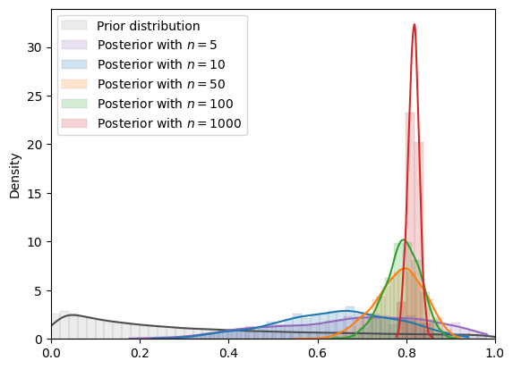
_images/3d4ced27eb5ea876a8af7e6feb2dafea556f18e8895965adc68ac96b2fe88e7a.png — Fig. 18.10 MCMC density (log normal prior)#

# von Mises
example_CLASS = VONMISES
print(
    f"=======INFO=======\nParameters: {example_CLASS.param}\nPrior Dist: {example_CLASS.name_dist}"
)
print("\nNOTE: Shifted von Mises")
example_plotCLASS = BayesianInferencePlot(
    true_theta, num_list, example_CLASS
    )
MCMC_plot(
    example_plotCLASS, num_samples=MCMC_num_samples
)

=======INFO=======
Parameters: 10
Prior Dist: vonMises

NOTE: Shifted von Mises

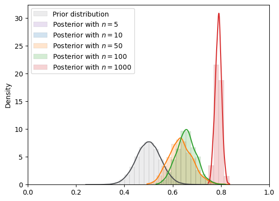
_images/d3852e92bd13ec5935092d0876c19785f189dc181b77973d89810207283a73b0.png — Fig. 18.11 MCMC density (von Mises prior)#

# Laplace
example_CLASS = LAPLACE
print(
    f"=======INFO=======\nParameters: {example_CLASS.param}\nPrior Dist: {example_CLASS.name_dist}"
)
example_plotCLASS = BayesianInferencePlot(
    true_theta, num_list, example_CLASS
    )
MCMC_plot(
    example_plotCLASS, num_samples=MCMC_num_samples
)

=======INFO=======
Parameters: (0.5, 0.07)
Prior Dist: laplace

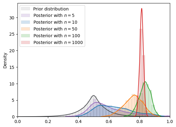
_images/a4545631793ead3243e3bbebf20f91fb643227f3aca4909ca807bdec642148cc.png — Fig. 18.12 MCMC density (Laplace prior)#

18.6.2. VI#

To get more accuracy we will now increase the number of steps for Variational Inference (VI)

SVI_num_steps = 50000

18.6.2.1. VI with a truncated normal guide#

# Uniform
example_CLASS = BayesianInference(param=(0, 1), name_dist="uniform")
print(
    f"=======INFO=======\nParameters: {example_CLASS.param}\nPrior Dist: {example_CLASS.name_dist}"
)
example_plotCLASS = BayesianInferencePlot(
    true_theta, num_list, example_CLASS
    )
SVI_plot(
    example_plotCLASS, guide_dist="normal", n_steps=SVI_num_steps
)

=======INFO=======
Parameters: (0, 1)
Prior Dist: uniform

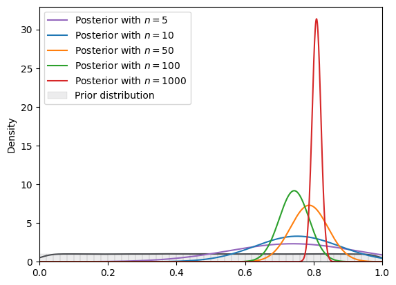
_images/c12061fd0ca45a7f28bf91f0b8d84c5f301d2136521fb157eab4d76681e2a02e.png — Fig. 18.13 SVI density (uniform prior, normal guide)#

# log normal
example_CLASS = LOGNORMAL
print(
    f"=======INFO=======\nParameters: {example_CLASS.param}\nPrior Dist: {example_CLASS.name_dist}"
)
example_plotCLASS = BayesianInferencePlot(
    true_theta, num_list, example_CLASS
    )
SVI_plot(
    example_plotCLASS, guide_dist="normal", n_steps=SVI_num_steps
)

=======INFO=======
Parameters: (0, 2)
Prior Dist: lognormal

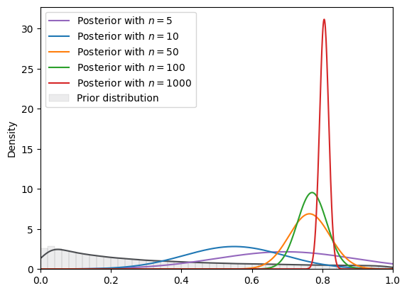
_images/809b27bf54a5d047a903775ca505b116d52877c72c363c677a25c741b8a9a6aa.png — Fig. 18.14 SVI density (log normal prior, normal guide)#

# Laplace
example_CLASS = LAPLACE
print(
    f"=======INFO=======\nParameters: {example_CLASS.param}\nPrior Dist: {example_CLASS.name_dist}"
)
example_plotCLASS = BayesianInferencePlot(
    true_theta, num_list, example_CLASS
    )
SVI_plot(
    example_plotCLASS, guide_dist="normal", n_steps=SVI_num_steps
)

=======INFO=======
Parameters: (0.5, 0.07)
Prior Dist: laplace

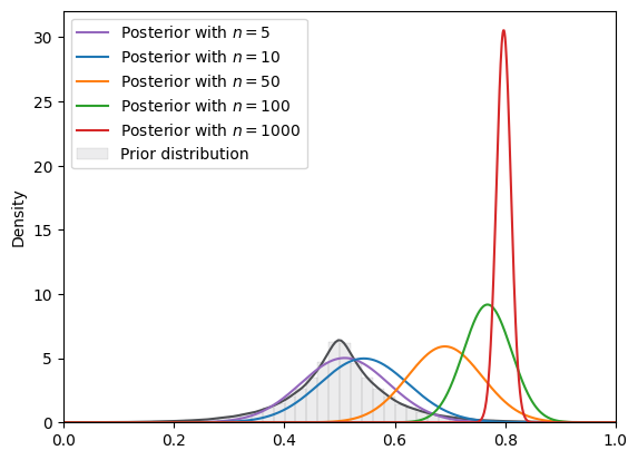
_images/732b8abf490847543a389a7d81ab650011d86e0565ba1c19a06339d45b5faeff.png — Fig. 18.15 SVI density (Laplace prior, normal guide)#

18.6.2.2. Variational inference with a Beta guide distribution#

# uniform
example_CLASS = STD_UNIFORM
print(
    f"=======INFO=======\nParameters: {example_CLASS.param}\nPrior Dist: {example_CLASS.name_dist}"
)
example_plotCLASS = BayesianInferencePlot(
    true_theta, num_list, example_CLASS
    )
SVI_plot(
    example_plotCLASS, guide_dist="beta", n_steps=SVI_num_steps
)

=======INFO=======
Parameters: (0, 1)
Prior Dist: uniform

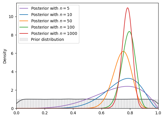
_images/bbcf97c693baaae73bf9c0bbdf2523775c2f1eb5e6015f7e0ad21e5e320e6548.png — Fig. 18.16 SVI density (uniform prior, Beta guide)#

# log normal
example_CLASS = LOGNORMAL
print(
    f"=======INFO=======\nParameters: {example_CLASS.param}\nPrior Dist: {example_CLASS.name_dist}"
)
example_plotCLASS = BayesianInferencePlot(
    true_theta, num_list, example_CLASS
    )
SVI_plot(
    example_plotCLASS, guide_dist="beta", n_steps=SVI_num_steps
)

=======INFO=======
Parameters: (0, 2)
Prior Dist: lognormal

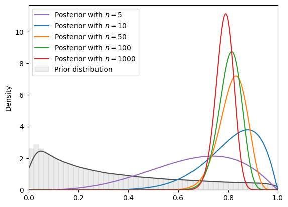
_images/96a20247e74222272a335b854dca37b2deedb63d9ffac6c496048ef6058825db.png — Fig. 18.17 SVI density (log normal prior, Beta guide)#

# von Mises
example_CLASS = VONMISES
print(
    f"=======INFO=======\nParameters: {example_CLASS.param}\nPrior Dist: {example_CLASS.name_dist}"
)
print("Shifted von Mises")
example_plotCLASS = BayesianInferencePlot(
    true_theta, num_list, example_CLASS
    )
SVI_plot(
    example_plotCLASS, guide_dist="beta", n_steps=SVI_num_steps
)

=======INFO=======
Parameters: 10
Prior Dist: vonMises
Shifted von Mises

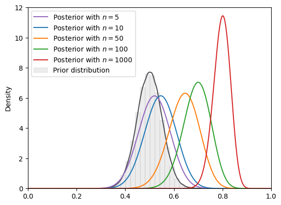
_images/1cb6a07f31fd73abc6a97ea111e765d0719f4058e6310d1773b842f82e1fea60.png — Fig. 18.18 SVI density (von Mises prior, Beta guide)#

# Laplace
example_CLASS = LAPLACE
print(
    f"=======INFO=======\nParameters: {example_CLASS.param}\nPrior Dist: {example_CLASS.name_dist}"
)
example_plotCLASS = BayesianInferencePlot(
    true_theta, num_list, example_CLASS
    )
SVI_plot(
    example_plotCLASS, guide_dist="beta", n_steps=SVI_num_steps
)

=======INFO=======
Parameters: (0.5, 0.07)
Prior Dist: laplace

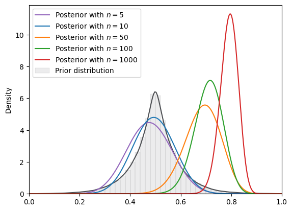
_images/4a9ef12383dbc1f598964cb4e714e3a203df7c111616eb6de096c9523eac057d.png — Fig. 18.19 SVI density (Laplace prior, Beta guide)#