8. Elementary Probability with Matrices#

This lecture uses matrix algebra to illustrate some basic ideas about probability theory.

After introducing underlying objects, we’ll use matrices and vectors to describe probability distributions.

Among concepts that we’ll be studying include

a joint probability distribution
marginal distributions associated with a given joint distribution
conditional probability distributions
statistical independence of two random variables
joint distributions associated with a prescribed set of marginal distributions
- couplings
- copulas
the probability distribution of a sum of two independent random variables
- convolution of marginal distributions
parameters that define a probability distribution
sufficient statistics as data summaries

We’ll use a matrix to represent a bivariate or multivariate probability distribution and a vector to represent a univariate probability distribution

This companion lecture describes some popular probability distributions and describes how to use Python to sample from them.

In addition to what’s in Anaconda, this lecture will need the following libraries:

!pip install prettytable

As usual, we’ll start with some imports

import numpy as np
import matplotlib.pyplot as plt
import prettytable as pt
from mpl_toolkits.mplot3d import Axes3D
from matplotlib_inline.backend_inline import set_matplotlib_formats
set_matplotlib_formats('retina')

8.1. Sketch of Basic Concepts#

We’ll briefly define what we mean by a probability space, a probability measure, and a random variable.

For most of this lecture, we sweep these objects into the background

Note

Nevertheless, they’ll be lurking beneath induced distributions of random variables that we’ll focus on here. These deeper objects are essential for defining and analysing the concepts of stationarity and ergodicity that underly laws of large numbers. For a relatively nontechnical presentation of some of these results see this chapter from Lars Peter Hansen and Thomas J. Sargent’s online monograph titled “Risk, Uncertainty, and Values”:https://lphansen.github.io/QuantMFR/book/1_stochastic_processes.html.

Let $Ω$ be a set of possible underlying outcomes and let $ω \in Ω$ be a particular underlying outcomes.

Let $G \subset Ω$ be a subset of $Ω$ .

Let $F$ be a collection of such subsets $G \subset Ω$ .

The pair $Ω, F$ forms our probability space on which we want to put a probability measure.

A probability measure $μ$ maps a set of possible underlying outcomes $G \in F$ into a scalar number between $0$ and $1$

this is the “probability” that $X$ belongs to $A$ , denoted by $Prob {X \in A}$ .

A random variable $X (ω)$ is a function of the underlying outcome $ω \in Ω$ .

The random variable $X (ω)$ has a probability distribution that is induced by the underlying probability measure $μ$ and the function $X (ω)$ :

(8.1)#

Prob (X \in A) = \int_{G} μ (ω) d ω

where $G$ is the subset of $Ω$ for which $X (ω) \in A$ .

We call this the induced probability distribution of random variable $X$ .

Instead of working explicitly with an underlying probability space $Ω, F$ and probability measure $μ$ , applied statisticians often proceed simply by specifying a form for an induced distribution for a random variable $X$ .

That is how we’ll proceed in this lecture and in many subsequent lectures.

8.2. What Does Probability Mean?#

Before diving in, we’ll say a few words about what probability theory means and how it connects to statistics.

We also touch on these topics in the quantecon lectures https://python.quantecon.org/prob_meaning.html and https://python.quantecon.org/navy_captain.html.

For much of this lecture we’ll be discussing fixed “population” probabilities.

These are purely mathematical objects.

To appreciate how statisticians connect probabilities to data, the key is to understand the following concepts:

A single draw from a probability distribution
Repeated independently and identically distributed (i.i.d.) draws of “samples” or “realizations” from the same probability distribution
A statistic defined as a function of a sequence of samples
An empirical distribution or histogram (a binned empirical distribution) that records observed relative frequencies
The idea that a population probability distribution is what we anticipate relative frequencies will be in a long sequence of i.i.d. draws. Here the following mathematical machinery makes precise what is meant by anticipated relative frequencies
- Law of Large Numbers (LLN)
- Central Limit Theorem (CLT)

Scalar example

Let $X$ be a scalar random variable that takes on the $I$ possible values $0, 1, 2, \dots, I - 1$ with probabilities

P r o b (X = i) = f_{i},

where

f_{i} ⩾ 0, \sum_{i} f_{i} = 1 .

We sometimes write

X \sim {f_{i}}_{i = 0}^{I - 1}

as a short-hand way of saying that the random variable $X$ is described by the probability distribution ${f_{i}}_{i = 0}^{I - 1}$ .

Consider drawing a sample $x_{0}, x_{1}, \dots, x_{N - 1}$ of $N$ independent and identically distributoed draws of $X$ .

What do the “identical” and “independent” mean in IID or iid (“identically and independently distributed”)?

“identical” means that each draw is from the same distribution.
“independent” means that joint distribution equal products of marginal distributions, i.e.,

\begin{array}{r} \begin{aligned} Prob {x_{0} = i_{0}, x_{1} = i_{1}, \dots, x_{N - 1} = i_{N - 1}} & = Prob {x_{0} = i_{0}} \cdot \dots \cdot Prob {x_{I - 1} = i_{I - 1}} \\ = f_{i_{0}} f_{i_{1}} \cdot \dots \cdot f_{i_{N - 1}} \end{aligned} \end{array}

We define an empirical distribution as follows.

For each $i = 0, \dots, I - 1$ , let

\begin{array}{r} \begin{aligned} N_{i} & = number of times X = i, \\ N & = \sum_{i = 0}^{I - 1} N_{i} total number of draws, \\ \tilde{f_{i}} & = \frac{N_{i}}{N} \sim frequency of draws for which X = i \end{aligned} \end{array}

Key concepts that connect probability theory with statistics are laws of large numbers and central limit theorems

LLN:

A Law of Large Numbers (LLN) states that $\tilde{f_{i}} \to f_{i} as N \to \infty$

CLT:

A Central Limit Theorem (CLT) describes a rate at which $\tilde{f_{i}} \to f_{i}$

Remarks

For “frequentist” statisticians, anticipated relative frequency is all that a probability distribution means.
But for a Bayesian it means something else – something partly subjective and purely personal.
- we say “partly” because a Bayesian also pays attention to relative frequencies

8.3. Representing Probability Distributions#

A probability distribution $Prob (X \in A)$ can be described by its cumulative distribution function (CDF)

F_{X} (x) = Prob {X \leq x} .

Sometimes, but not always, a random variable can also be described by density function $f (x)$ that is related to its CDF by

Prob {X \in B} = \int_{t \in B} f (t) d t

F (x) = \int_{- \infty}^{x} f (t) d t

Here $B$ is a set of possible $X$ ’s whose probability of occurring we want to compute.

When a probability density exists, a probability distribution can be characterized either by its CDF or by its density.

For a discrete-valued random variable

the number of possible values of $X$ is finite or countably infinite
we replace a density with a probability mass function, a non-negative sequence that sums to one
we replace integration with summation in the formula like (8.1) that relates a CDF to a probability mass function

In this lecture, we mostly discuss discrete random variables.

Doing this enables us to confine our tool set basically to linear algebra.

Later we’ll briefly discuss how to approximate a continuous random variable with a discrete random variable.

8.4. Univariate Probability Distributions#

We’ll devote most of this lecture to discrete-valued random variables, but we’ll say a few things about continuous-valued random variables.

8.4.1. Discrete random variable#

Let $X$ be a discrete random variable that takes possible values: $i = 0, 1, \dots, I - 1 = \bar{X}$ .

Here, we choose the maximum index $I - 1$ because of how this aligns nicely with Python’s index convention.

Define $f_{i} \equiv Prob {X = i}$ and assemble the non-negative vector

(8.2)#

\begin{array}{r} f = [\begin{array}{c} f_{0} \\ f_{1} \\ ⋮ \\ f_{I - 1} \end{array}] \end{array}

for which $f_{i} \in [0, 1]$ for each $i$ and $\sum_{i = 0}^{I - 1} f_{i} = 1$ .

This vector defines a probability mass function.

The distribution (8.2) has parameters ${f_{i}}_{i = 0, 1, \dots, I - 2}$ since $f_{I - 1} = 1 - \sum_{i = 0}^{I - 2} f_{i}$ .

These parameters pin down the shape of the distribution.

(Sometimes $I = \infty$ .)

Such a “non-parametric” distribution has as many “parameters” as there are possible values of the random variable.

We often work with special distributions that are characterized by a small number parameters.

In these special parametric distributions,

f_{i} = g (i; θ)

where $θ$ is a vector of parameters that is of much smaller dimension than $I$ .

Remarks:

A statistical model is a joint probability distribution characterized by a list of parameters
The concept of parameter is intimately related to the notion of sufficient statistic.
A statistic is a nonlinear function of a data set.
Sufficient statistics summarize all information that a data set contains about parameters of statistical model.
- Note that a sufficient statistic corresponds to a particular statistical model.
- Sufficient statistics are key tools that AI uses to summarize or compress a big data set.
R. A. Fisher provided a rigorous definition of information – see https://en.wikipedia.org/wiki/Fisher_information

An example of a parametric probability distribution is a geometric distribution.

It is described by

f_{i} = Prob {X = i} = (1 - λ) λ^{i}, λ \in [0, 1], i = 0, 1, 2, \dots

Evidently, $\sum_{i = 0}^{\infty} f_{i} = 1$ .

Let $θ$ be a vector of parameters of the distribution described by $f$ , then

f_{i} (θ) \geq 0, \sum_{i = 0}^{\infty} f_{i} (θ) = 1

8.4.2. Continuous random variable#

Let $X$ be a continous random variable that takes values $X \in \tilde{X} \equiv [X_{U}, X_{L}]$ whose distributions have parameters $θ$ .

Prob {X \in A} = \int_{x \in A} f (x; θ) d x; f (x; θ) \geq 0

where $A$ is a subset of $\tilde{X}$ and

Prob {X \in \tilde{X}} = 1

8.5. Bivariate Probability Distributions#

We’ll now discuss a bivariate joint distribution.

To begin, we restrict ourselves to two discrete random variables.

Let $X, Y$ be two discrete random variables that take values:

X \in {0, \dots, I - 1}

Y \in {0, \dots, J - 1}

Then their joint distribution is described by a matrix

F_{I \times J} = [f_{i j}]_{i \in {0, \dots, I - 1}, j \in {0, \dots, J - 1}}

whose elements are

f_{i j} = Prob {X = i, Y = j} \geq 0

where

\sum_{i} \sum_{j} f_{i j} = 1

8.6. Marginal Probability Distributions#

The joint distribution induce marginal distributions

Prob {X = i} = \sum_{j = 0}^{J - 1} f_{i j} = μ_{i}, i = 0, \dots, I - 1

Prob {Y = j} = \sum_{i = 0}^{I - 1} f_{i j} = ν_{j}, j = 0, \dots, J - 1

For example, let a joint distribution over $(X, Y)$ be

(8.3)#

\begin{array}{r} F = [\begin{array}{c} .25 & .1 \\ .15 & .5 \end{array}] \end{array}

The implied marginal distributions are:

\begin{array}{r} \begin{aligned} Prob {X = 0} & = .25 + .1 = .35 \\ Prob {X = 1} & = .15 + .5 = .65 \\ Prob {Y = 0} & = .25 + .15 = .4 \\ Prob {Y = 1} & = .1 + .5 = .6 \end{aligned} \end{array}

Digression: If two random variables $X, Y$ are continuous and have joint density $f (x, y)$ , then marginal distributions can be computed by

\begin{array}{r} \begin{aligned} f (x) & = \int_{R} f (x, y) d y \\ f (y) & = \int_{R} f (x, y) d x \end{aligned} \end{array}

8.7. Conditional Probability Distributions#

Conditional probabilities are defined according to

Prob {A ∣ B} = \frac{Prob {A \cap B}}{Prob {B}}

where $A, B$ are two events.

For a pair of discrete random variables, we have the conditional distribution

Prob {X = i | Y = j} = \frac{f_{i j}}{\sum_{i} f_{i j}} = \frac{Prob {X = i, Y = j}}{Prob {Y = j}}

where $i = 0, \dots, I - 1, j = 0, \dots, J - 1$ .

Note that

\sum_{i} Prob {X_{i} = i | Y_{j} = j} = \frac{\sum_{i} f_{i j}}{\sum_{i} f_{i j}} = 1

Remark: The mathematics of conditional probability implies:

(8.4)#

Prob {X = i | Y = j} = \frac{Prob {X = i, Y = j}}{Prob {Y = j}} = \frac{Prob {Y = j | X = i} Prob {X = i}}{Prob {Y = j}}

Note

Formula (8.4) is also what a Bayesian calls Bayes’ Law. A Bayesian statistician regards marginal probability distribution $Prob (X = i), i = 1, \dots, J$ as a prior distribution that describes his personal subjective beliefs about $X$ . He then interprets formula (8.4) as a procedure for constructing a posterior distribution that describes how he would revise his subjective beliefs after observing that $Y$ equals $j$ .

For the joint distribution (8.3)

Prob {X = 0 | Y = 1} = \frac{.1}{.1 + .5} = \frac{.1}{.6}

8.8. Transition Probability Matrix#

Consider the following joint probability distribution of two random variables.

Let $X, Y$ be discrete random variables with joint distribution

Prob {X = i, Y = j} = ρ_{i j}

where $i = 0, \dots, I - 1; j = 0, \dots, J - 1$ and

\sum_{i} \sum_{j} ρ_{i j} = 1, ρ_{i j} ⩾ 0.

An associated conditional distribution is

Prob {Y = i | X = j} = \frac{ρ_{i j}}{\sum_{j} ρ_{i j}} = \frac{Prob {Y = j, X = i}}{Prob {X = i}}

We can define a transition probability matrix $P$ with $i, j$ component

p_{i j} = Prob {Y = j | X = i} = \frac{ρ_{i j}}{\sum_{j} ρ_{i j}}

where

\begin{array}{r} [\begin{array}{c} p_{11} & p_{12} \\ p_{21} & p_{22} \end{array}] \end{array}

The first row is the probability that $Y = j, j = 0, 1$ conditional on $X = 0$ .

The second row is the probability that $Y = j, j = 0, 1$ conditional on $X = 1$ .

Note that

$\sum_{j} ρ_{i j} = \frac{\sum_{j} ρ_{i j}}{\sum_{j} ρ_{i j}} = 1$ , so each row of the transition matrix $P$ is a probability distribution (not so for each column).

8.9. Application: Forecasting a Time Series#

Suppose that there are two time periods.

$t = 0$ “today”
$t = 1$ “tomorrow”

Let $X (0)$ be a random variable to be realized at $t = 0$ , $X (1)$ be a random variable to be realized at $t = 1$ .

Suppose that

\begin{array}{r} \begin{aligned} Prob {X (0) = i, X (1) = j} & = f_{i j} \geq 0 ， i = 0, \dots, I - 1 \\ \sum_{i} \sum_{j} f_{i j} & = 1 \end{aligned} \end{array}

$f_{i j}$ is a joint distribution over $[X (0), X (1)]$ .

A conditional distribution is

Prob {X (1) = j | X (0) = i} = \frac{f_{i j}}{\sum_{j} f_{i j}}

Remark:

This formula is a workhorse for applied economic forecasters.

8.10. Statistical Independence#

Random variables X and Y are statistically independent if

Prob {X = i, Y = j} = f_{i} g_{j}

where

\begin{aligned} Prob {X = i} & = f_{i} \geq 0 ， \sum f_{i} = 1 \\ Prob {Y = j} & = g_{j} \geq 0 ， \sum g_{j} = 1 \end{aligned}

Conditional distributions are

\begin{array}{r} \begin{aligned} Prob {X = i | Y = j} & = \frac{f_{i} g_{j}}{\sum_{i} f_{i} g_{j}} = \frac{f_{i} g_{j}}{g_{j}} = f_{i} \\ Prob {Y = j | X = i} & = \frac{f_{i} g_{j}}{\sum_{j} f_{i} g_{j}} = \frac{f_{i} g_{j}}{f_{i}} = g_{j} \end{aligned} \end{array}

8.11. Means and Variances#

The mean and variance of a discrete random variable $X$ are

\begin{array}{r} \begin{aligned} μ_{X} & \equiv E [X] = \sum_{k} k Prob {X = k} \\ σ_{X}^{2} & \equiv D [X] = \sum_{k} {(k - E [X])}^{2} Prob {X = k} \end{aligned} \end{array}

A continuous random variable having density $f_{X} (x)$ ) has mean and variance

\begin{array}{r} \begin{aligned} μ_{X} & \equiv E [X] = \int_{- \infty}^{\infty} x f_{X} (x) d x \\ σ_{X}^{2} \equiv D [X] & = E [{(X - μ_{X})}^{2}] = \int_{- \infty}^{\infty} {(x - μ_{X})}^{2} f_{X} (x) d x \end{aligned} \end{array}

8.12. Matrix Representations of Some Bivariate Distributions#

Let’s use matrices to represent a joint distribution, conditional distribution, marginal distribution, and the mean and variance of a bivariate random variable.

The table below illustrates a probability distribution for a bivariate random variable.

\begin{array}{r} F = [f_{i j}] = [\begin{array}{cc} 0.3 & 0.2 \\ 0.1 & 0.4 \end{array}] \end{array}

Marginal distributions are

Prob (X = i) = \sum_{j} f_{i j} = u_{i}

Prob (Y = j) = \sum_{i} f_{i j} = v_{j}

Sampling:

Let’s write some Python code that let’s us draw some long samples and compute relative frequencies.

The code will let us check whether the “sampling” distribution agrees with the “population” distribution - confirming that the population distribution correctly tells us the relative frequencies that we should expect in a large sample.

# specify parameters
xs = np.array([0, 1])
ys = np.array([10, 20])
f = np.array([[0.3, 0.2], [0.1, 0.4]])
f_cum = np.cumsum(f)

# draw random numbers
p = np.random.rand(1_000_000)
x = np.vstack([xs[1]*np.ones(p.shape), ys[1]*np.ones(p.shape)])
# map to the bivariate distribution

x[0, p < f_cum[2]] = xs[1]
x[1, p < f_cum[2]] = ys[0]

x[0, p < f_cum[1]] = xs[0]
x[1, p < f_cum[1]] = ys[1]

x[0, p < f_cum[0]] = xs[0]
x[1, p < f_cum[0]] = ys[0]
print(x)

[[ 1.  0.  1. ...  0.  0.  1.]
 [20. 10. 20. ... 20. 10. 10.]]

Note

To generate random draws from the joint distribution $F$ , we use the inverse CDF technique described in this companion lecture.

# marginal distribution
xp = np.sum(x[0, :] == xs[0])/1_000_000
yp = np.sum(x[1, :] == ys[0])/1_000_000

# print output
print("marginal distribution for x")
xmtb = pt.PrettyTable()
xmtb.field_names = ['x_value', 'x_prob']
xmtb.add_row([xs[0], xp])
xmtb.add_row([xs[1], 1-xp])
print(xmtb)

print("\nmarginal distribution for y")
ymtb = pt.PrettyTable()
ymtb.field_names = ['y_value', 'y_prob']
ymtb.add_row([ys[0], yp])
ymtb.add_row([ys[1], 1-yp])
print(ymtb)

marginal distribution for x
+---------+---------------------+
| x_value |        x_prob       |
+---------+---------------------+
|    0    |       0.500384      |
|    1    | 0.49961599999999995 |
+---------+---------------------+

marginal distribution for y
+---------+----------+
| y_value |  y_prob  |
+---------+----------+
|    10   | 0.400001 |
|    20   | 0.599999 |
+---------+----------+

# conditional distributions
xc1 = x[0, x[1, :] == ys[0]]
xc2 = x[0, x[1, :] == ys[1]]
yc1 = x[1, x[0, :] == xs[0]]
yc2 = x[1, x[0, :] == xs[1]]

xc1p = np.sum(xc1 == xs[0])/len(xc1)
xc2p = np.sum(xc2 == xs[0])/len(xc2)
yc1p = np.sum(yc1 == ys[0])/len(yc1)
yc2p = np.sum(yc2 == ys[0])/len(yc2)

# print output
print("conditional distribution for x")
xctb = pt.PrettyTable()
xctb.field_names = ['y_value', 'prob(x=0)', 'prob(x=1)']
xctb.add_row([ys[0], xc1p, 1-xc1p])
xctb.add_row([ys[1], xc2p, 1-xc2p])
print(xctb)

print("\nconditional distribution for y")
yctb = pt.PrettyTable()
yctb.field_names = ['x_value',  'prob(y=10)', 'prob(y=20)']
yctb.add_row([xs[0], yc1p, 1-yc1p])
yctb.add_row([xs[1], yc2p, 1-yc2p])
print(yctb)

conditional distribution for x
+---------+--------------------+--------------------+
| y_value |     prob(x=0)      |     prob(x=1)      |
+---------+--------------------+--------------------+
|    10   | 0.7501806245484386 | 0.2498193754515614 |
|    20   | 0.3338522230870385 | 0.6661477769129616 |
+---------+--------------------+--------------------+

conditional distribution for y
+---------+---------------------+--------------------+
| x_value |      prob(y=10)     |     prob(y=20)     |
+---------+---------------------+--------------------+
|    0    |  0.5996854415808659 | 0.4003145584191341 |
|    1    | 0.20000960737846665 | 0.7999903926215334 |
+---------+---------------------+--------------------+

Let’s calculate population marginal and conditional probabilities using matrix algebra.

\begin{array}{r} [\begin{array}{cccccc} ⋮ & y_{1} & y_{2} & ⋮ & x \\ \dots & ⋮ & \dots & \dots & ⋮ & \dots \\ x_{1} & ⋮ & 0.3 & 0.2 & ⋮ & 0.5 \\ x_{2} & ⋮ & 0.1 & 0.4 & ⋮ & 0.5 \\ \dots & ⋮ & \dots & \dots & ⋮ & \dots \\ y & ⋮ & 0.4 & 0.6 & ⋮ & 1 \end{array}] \end{array}

$⟹$

(1) Marginal distribution:

\begin{array}{r} [\begin{array}{cccccc} v a r & ⋮ & v a r_{1} & v a r_{2} \\ \dots & ⋮ & \dots & \dots \\ x & ⋮ & 0.5 & 0.5 \\ \dots & ⋮ & \dots & \dots \\ y & ⋮ & 0.4 & 0.6 \end{array}] \end{array}

(2) Conditional distribution:

\begin{array}{r} [\begin{array}{cccccc} x & ⋮ & x_{1} & x_{2} \\ \dots \dots \dots & ⋮ & \dots \dots \dots & \dots \dots \dots \\ y = y_{1} & ⋮ & \frac{0.3}{0.4} = 0.75 & \frac{0.1}{0.4} = 0.25 \\ \dots \dots \dots & ⋮ & \dots \dots \dots & \dots \dots \dots \\ y = y_{2} & ⋮ & \frac{0.2}{0.6} \approx 0.33 & \frac{0.4}{0.6} \approx 0.67 \end{array}] \end{array}

\begin{array}{r} [\begin{array}{cccccc} y & ⋮ & y_{1} & y_{2} \\ \dots \dots \dots & ⋮ & \dots \dots \dots & \dots \dots \dots \\ x = x_{1} & ⋮ & \frac{0.3}{0.5} = 0.6 & \frac{0.2}{0.5} = 0.4 \\ \dots \dots \dots & ⋮ & \dots \dots \dots & \dots \dots \dots \\ x = x_{2} & ⋮ & \frac{0.1}{0.5} = 0.2 & \frac{0.4}{0.5} = 0.8 \end{array}] \end{array}

These population objects closely resemble the sample counterparts computed above.

Let’s wrap some of the functions we have used in a Python class that will let us generate and sample from a discrete bivariate joint distribution.

class discrete_bijoint:

    def __init__(self, f, xs, ys):
        '''initialization
        -----------------
        parameters:
        f: the bivariate joint probability matrix
        xs: values of x vector
        ys: values of y vector
        '''
        self.f, self.xs, self.ys = f, xs, ys

    def joint_tb(self):
        '''print the joint distribution table'''
        xs = self.xs
        ys = self.ys
        f = self.f
        jtb = pt.PrettyTable()
        jtb.field_names = ['x_value/y_value', *ys, 'marginal sum for x']
        for i in range(len(xs)):
            jtb.add_row([xs[i], *f[i, :], np.sum(f[i, :])])
        jtb.add_row(['marginal_sum for y', *np.sum(f, 0), np.sum(f)])
        print("\nThe joint probability distribution for x and y\n", jtb)
        self.jtb = jtb

    def draw(self, n):
        '''draw random numbers
        ----------------------
        parameters:
        n: number of random numbers to draw
        '''
        xs = self.xs
        ys = self.ys
        f_cum = np.cumsum(self.f)
        p = np.random.rand(n)
        x = np.empty([2, p.shape[0]])
        lf = len(f_cum)
        lx = len(xs)-1
        ly = len(ys)-1
        for i in range(lf):
            x[0, p < f_cum[lf-1-i]] = xs[lx]
            x[1, p < f_cum[lf-1-i]] = ys[ly]
            if ly == 0:
                lx -= 1
                ly = len(ys)-1
            else:
                ly -= 1
        self.x = x
        self.n = n

    def marg_dist(self):
        '''marginal distribution'''
        x = self.x
        xs = self.xs
        ys = self.ys
        n = self.n
        xmp = [np.sum(x[0, :] == xs[i])/n for i in range(len(xs))]
        ymp = [np.sum(x[1, :] == ys[i])/n for i in range(len(ys))]

        # print output
        xmtb = pt.PrettyTable()
        ymtb = pt.PrettyTable()
        xmtb.field_names = ['x_value', 'x_prob']
        ymtb.field_names = ['y_value', 'y_prob']
        for i in range(max(len(xs), len(ys))):
            if i < len(xs):
                xmtb.add_row([xs[i], xmp[i]])
            if i < len(ys):
                ymtb.add_row([ys[i], ymp[i]])
        xmtb.add_row(['sum', np.sum(xmp)])
        ymtb.add_row(['sum', np.sum(ymp)])
        print("\nmarginal distribution for x\n", xmtb)
        print("\nmarginal distribution for y\n", ymtb)

        self.xmp = xmp
        self.ymp = ymp

    def cond_dist(self):
        '''conditional distribution'''
        x = self.x
        xs = self.xs
        ys = self.ys
        n = self.n
        xcp = np.empty([len(ys), len(xs)])
        ycp = np.empty([len(xs), len(ys)])
        for i in range(max(len(ys), len(xs))):
            if i < len(ys):
                xi = x[0, x[1, :] == ys[i]]
                idx = xi.reshape(len(xi), 1) == xs.reshape(1, len(xs))
                xcp[i, :] = np.sum(idx, 0)/len(xi)
            if i < len(xs):
                yi = x[1, x[0, :] == xs[i]]
                idy = yi.reshape(len(yi), 1) == ys.reshape(1, len(ys))
                ycp[i, :] = np.sum(idy, 0)/len(yi)

        # print output
        xctb = pt.PrettyTable()
        yctb = pt.PrettyTable()
        xctb.field_names = ['x_value', *xs, 'sum']
        yctb.field_names = ['y_value', *ys, 'sum']
        for i in range(max(len(xs), len(ys))):
            if i < len(ys):
                xctb.add_row([ys[i], *xcp[i], np.sum(xcp[i])])
            if i < len(xs):
                yctb.add_row([xs[i], *ycp[i], np.sum(ycp[i])])
        print("\nconditional distribution for x\n", xctb)
        print("\nconditional distribution for y\n", yctb)

        self.xcp = xcp
        self.xyp = ycp

Let’s apply our code to some examples.

Example 1

# joint
d = discrete_bijoint(f, xs, ys)
d.joint_tb()

The joint probability distribution for x and y
 +--------------------+-----+--------------------+--------------------+
|  x_value/y_value   |  10 |         20         | marginal sum for x |
+--------------------+-----+--------------------+--------------------+
|         0          | 0.3 |        0.2         |        0.5         |
|         1          | 0.1 |        0.4         |        0.5         |
| marginal_sum for y | 0.4 | 0.6000000000000001 |        1.0         |
+--------------------+-----+--------------------+--------------------+

# sample marginal
d.draw(1_000_000)
d.marg_dist()

marginal distribution for x
 +---------+----------+
| x_value |  x_prob  |
+---------+----------+
|    0    | 0.499565 |
|    1    | 0.500435 |
|   sum   |   1.0    |
+---------+----------+

marginal distribution for y
 +---------+----------+
| y_value |  y_prob  |
+---------+----------+
|    10   | 0.399873 |
|    20   | 0.600127 |
|   sum   |   1.0    |
+---------+----------+

# sample conditional
d.cond_dist()

conditional distribution for x
 +---------+--------------------+--------------------+-----+
| x_value |         0          |         1          | sum |
+---------+--------------------+--------------------+-----+
|    10   | 0.7498955918504125 | 0.2501044081495875 | 1.0 |
|    20   | 0.3327662311477404 | 0.6672337688522596 | 1.0 |
+---------+--------------------+--------------------+-----+

conditional distribution for y
 +---------+---------------------+---------------------+-----+
| y_value |          10         |          20         | sum |
+---------+---------------------+---------------------+-----+
|    0    |  0.6002482159478747 | 0.39975178405212536 | 1.0 |
|    1    | 0.19984613386353872 |  0.8001538661364613 | 1.0 |
+---------+---------------------+---------------------+-----+

Example 2

xs_new = np.array([10, 20, 30])
ys_new = np.array([1, 2])
f_new = np.array([[0.2, 0.1], [0.1, 0.3], [0.15, 0.15]])
d_new = discrete_bijoint(f_new, xs_new, ys_new)
d_new.joint_tb()

The joint probability distribution for x and y
 +--------------------+---------------------+------+---------------------+
|  x_value/y_value   |          1          |  2   |  marginal sum for x |
+--------------------+---------------------+------+---------------------+
|         10         |         0.2         | 0.1  | 0.30000000000000004 |
|         20         |         0.1         | 0.3  |         0.4         |
|         30         |         0.15        | 0.15 |         0.3         |
| marginal_sum for y | 0.45000000000000007 | 0.55 |         1.0         |
+--------------------+---------------------+------+---------------------+

d_new.draw(1_000_000)
d_new.marg_dist()

marginal distribution for x
 +---------+----------+
| x_value |  x_prob  |
+---------+----------+
|    10   | 0.30058  |
|    20   | 0.399609 |
|    30   | 0.299811 |
|   sum   |   1.0    |
+---------+----------+

marginal distribution for y
 +---------+----------+
| y_value |  y_prob  |
+---------+----------+
|    1    | 0.449896 |
|    2    | 0.550104 |
|   sum   |   1.0    |
+---------+----------+

d_new.cond_dist()

conditional distribution for x
 +---------+---------------------+---------------------+---------------------+-----+
| x_value |          10         |          20         |          30         | sum |
+---------+---------------------+---------------------+---------------------+-----+
|    1    |  0.4453362554901577 | 0.22107998292938813 | 0.33358376158045416 | 1.0 |
|    2    | 0.18219282172098367 |  0.5456168288178236 |  0.2721903494611928 | 1.0 |
+---------+---------------------+---------------------+---------------------+-----+

conditional distribution for y
 +---------+---------------------+--------------------+-----+
| y_value |          1          |         2          | sum |
+---------+---------------------+--------------------+-----+
|    10   |  0.6665613147914032 | 0.3334386852085967 | 1.0 |
|    20   | 0.24890080053252053 | 0.7510991994674795 | 1.0 |
|    30   |  0.5005753624783613 | 0.4994246375216386 | 1.0 |
+---------+---------------------+--------------------+-----+

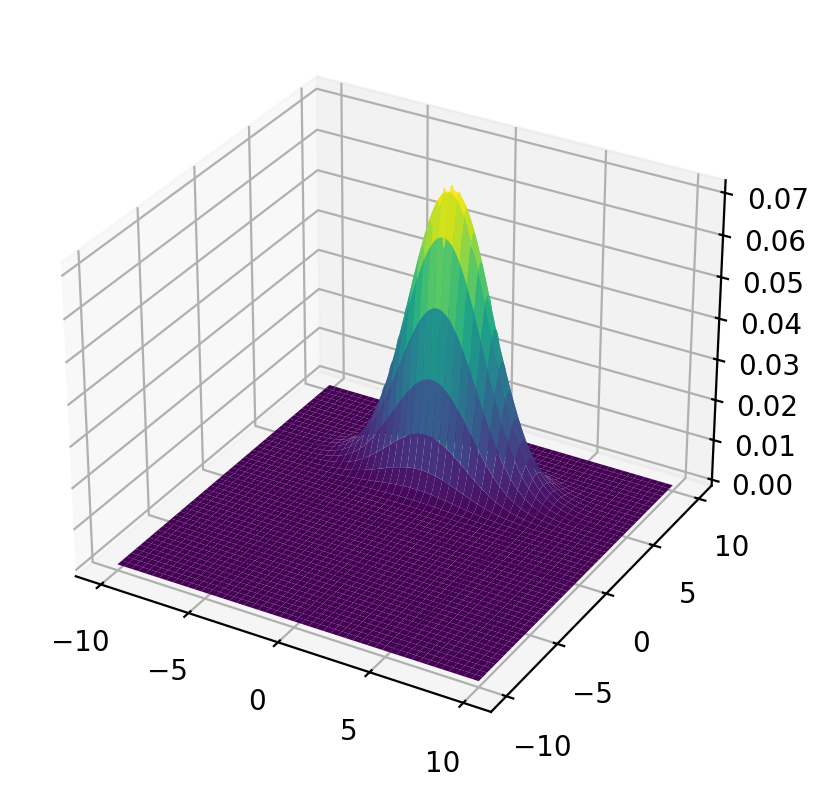
8.13. A Continuous Bivariate Random Vector#

A two-dimensional Gaussian distribution has joint density

f (x, y) = (2 π σ_{1} σ_{2} \sqrt{1 - ρ^{2}})^{- 1} \exp [- \frac{1}{2 (1 - ρ^{2})} (\frac{(x - μ_{1})^{2}}{σ_{1}^{2}} - \frac{2 ρ (x - μ_{1}) (y - μ_{2})}{σ_{1} σ_{2}} + \frac{(y - μ_{2})^{2}}{σ_{2}^{2}})]

\frac{1}{2 π σ_{1} σ_{2} \sqrt{1 - ρ^{2}}} \exp [- \frac{1}{2 (1 - ρ^{2})} (\frac{(x - μ_{1})^{2}}{σ_{1}^{2}} - \frac{2 ρ (x - μ_{1}) (y - μ_{2})}{σ_{1} σ_{2}} + \frac{(y - μ_{2})^{2}}{σ_{2}^{2}})]

We start with a bivariate normal distribution pinned down by

\begin{array}{r} μ = [\begin{array}{c} 0 \\ 5 \end{array}], Σ = [\begin{array}{cc} 5 & .2 \\ .2 & 1 \end{array}] \end{array}

# define the joint probability density function
def func(x, y, μ1=0, μ2=5, σ1=np.sqrt(5), σ2=np.sqrt(1), ρ=.2/np.sqrt(5*1)):
    A = (2 * np.pi * σ1 * σ2 * np.sqrt(1 - ρ**2))**(-1)
    B = -1 / 2 / (1 - ρ**2)
    C1 = (x - μ1)**2 / σ1**2
    C2 = 2 * ρ * (x - μ1) * (y - μ2) / σ1 / σ2
    C3 = (y - μ2)**2 / σ2**2
    return A * np.exp(B * (C1 - C2 + C3))

μ1 = 0
μ2 = 5
σ1 = np.sqrt(5)
σ2 = np.sqrt(1)
ρ = .2 / np.sqrt(5 * 1)

x = np.linspace(-10, 10, 1_000)
y = np.linspace(-10, 10, 1_000)
x_mesh, y_mesh = np.meshgrid(x, y, indexing="ij")

Joint Distribution

Let’s plot the population joint density.

# %matplotlib notebook

fig = plt.figure()
ax = plt.axes(projection='3d')

surf = ax.plot_surface(x_mesh, y_mesh, func(x_mesh, y_mesh), cmap='viridis')
plt.show()

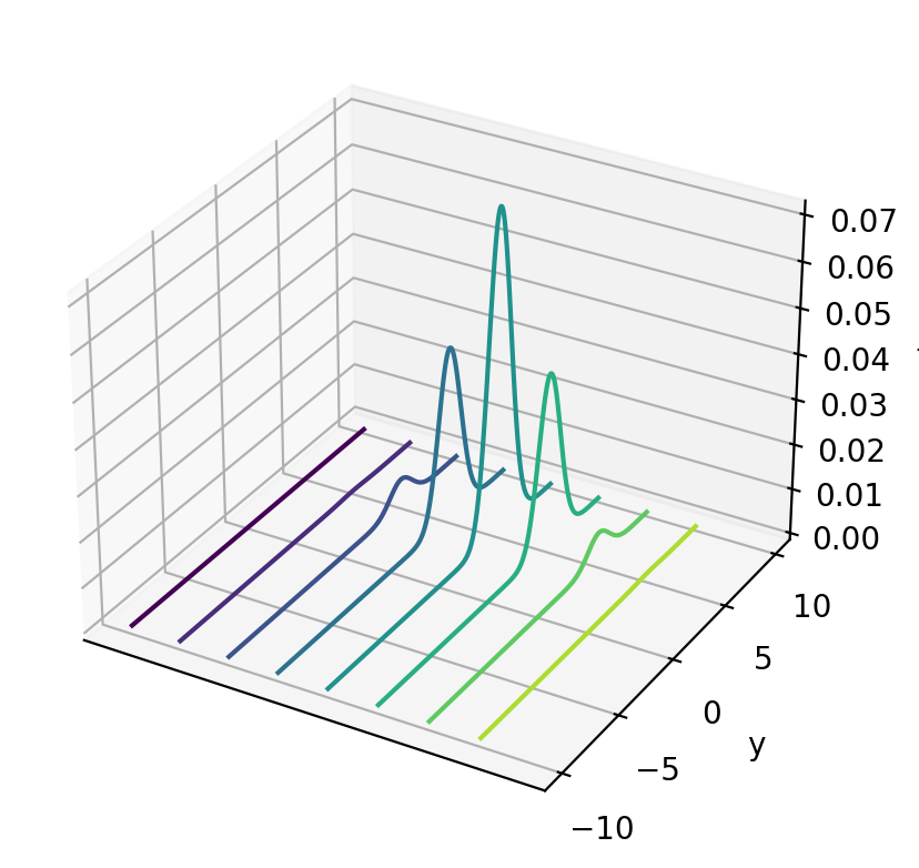
_images/74d39ba4e5a45f9e4656c2f3a5013176a786b05a1c82b2f84ebe589fa9cba3a4.png

# %matplotlib notebook

fig = plt.figure()
ax = plt.axes(projection='3d')

curve = ax.contour(x_mesh, y_mesh, func(x_mesh, y_mesh), zdir='x')
plt.ylabel('y')
ax.set_zlabel('f')
ax.set_xticks([])
plt.show()

_images/c99589206ffe472cc01658b23b0e6d07476eadaf0fff4104ba067979b02ff206.png

Next we can use a built-in numpy function to draw random samples, then calculate a sample marginal distribution from the sample mean and variance.

μ= np.array([0, 5])
σ= np.array([[5, .2], [.2, 1]])
n = 1_000_000
data = np.random.multivariate_normal(μ, σ, n)
x = data[:, 0]
y = data[:, 1]

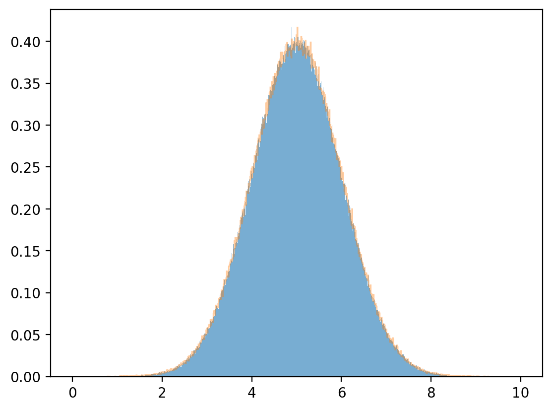
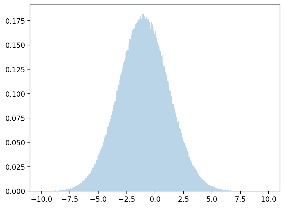
Marginal distribution

plt.hist(x, bins=1_000, alpha=0.6)
μx_hat, σx_hat = np.mean(x), np.std(x)
print(μx_hat, σx_hat)
x_sim = np.random.normal(μx_hat, σx_hat, 1_000_000)
plt.hist(x_sim, bins=1_000, alpha=0.4, histtype="step")
plt.show()

0.002760499570449984 2.2329239749158463

_images/82c494a757cf2cc8c5d9f5ac59743d2890875c643dd0be51b7901f990d35857d.png

plt.hist(y, bins=1_000, density=True, alpha=0.6)
μy_hat, σy_hat = np.mean(y), np.std(y)
print(μy_hat, σy_hat)
y_sim = np.random.normal(μy_hat, σy_hat, 1_000_000)
plt.hist(y_sim, bins=1_000, density=True, alpha=0.4, histtype="step")
plt.show()

5.000269373638193 0.9999825705690324

_images/b750ab9bc265c80b0923a13b19cb9f1caf937973331635740efbaabf310bfdc5.png

Conditional distribution

For a bivariate normal population distribution, the conditional distributions are also normal:

\begin{array}{r} \begin{aligned} [X | Y & = y] \sim N [μ_{X} + ρ σ_{X} \frac{y - μ_{Y}}{σ_{Y}}, σ_{X}^{2} (1 - ρ^{2})] \\ [Y | X & = x] \sim N [μ_{Y} + ρ σ_{Y} \frac{x - μ_{X}}{σ_{X}}, σ_{Y}^{2} (1 - ρ^{2})] \end{aligned} \end{array}

Note

Please see this quantecon lecture for more details.

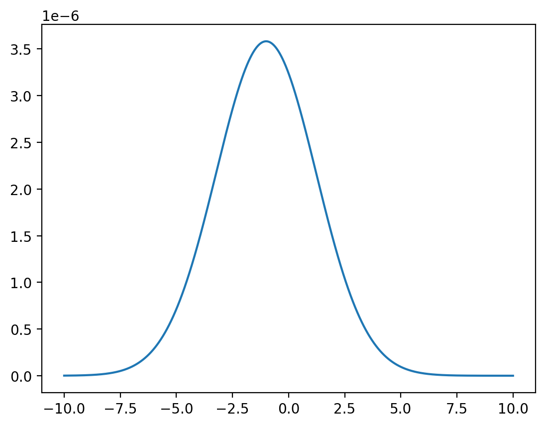
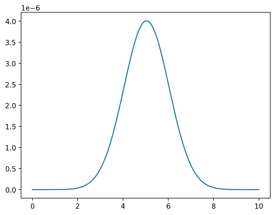
Let’s approximate the joint density by discretizing and mapping the approximating joint density into a matrix.

We can compute the discretized marginal density by just using matrix algebra and noting that

Prob {X = i | Y = j} = \frac{f_{i j}}{\sum_{i} f_{i j}}

Fix $y = 0$ .

# discretized marginal density
x = np.linspace(-10, 10, 1_000_000)
z = func(x, y=0) / np.sum(func(x, y=0))
plt.plot(x, z)
plt.show()

_images/25fc7d7a70197d3af618474a907b98fdf2592d3fe2ca462344d95dadab3c8a42.png

The mean and variance are computed by

\begin{array}{r} \begin{aligned} E [X | Y = j] & = \sum_{i} i P r o b {X = i | Y = j} = \sum_{i} i \frac{f_{i j}}{\sum_{i} f_{i j}} \\ D [X | Y = j] & = \sum_{i} {(i - μ_{X | Y = j})}^{2} \frac{f_{i j}}{\sum_{i} f_{i j}} \end{aligned} \end{array}

Let’s draw from a normal distribution with above mean and variance and check how accurate our approximation is.

# discretized mean
μx = np.dot(x, z)

# discretized standard deviation
σx = np.sqrt(np.dot((x - μx)**2, z))

# sample
zz = np.random.normal(μx, σx, 1_000_000)
plt.hist(zz, bins=300, density=True, alpha=0.3, range=[-10, 10])
plt.show()

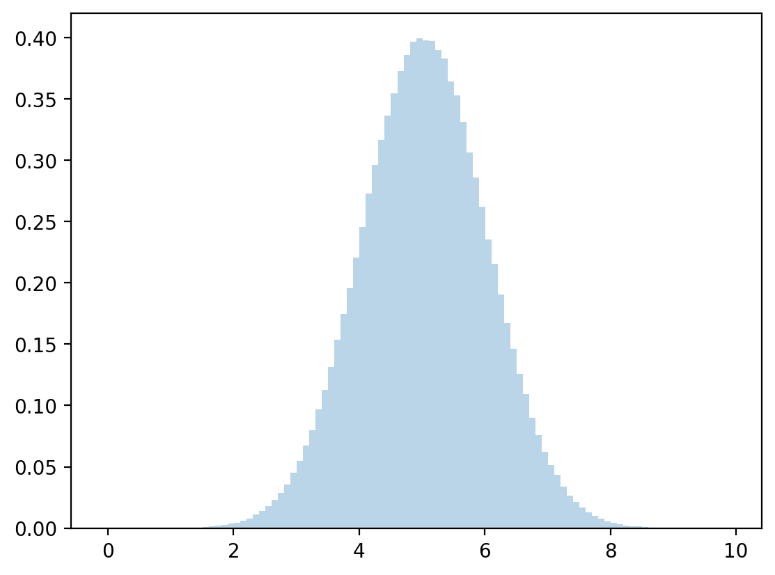
_images/3861f687accaa292193405da151c8aad87a0ebba5abc2859141e898a1ef8e5fd.png

Fix $x = 1$ .

y = np.linspace(0, 10, 1_000_000)
z = func(x=1, y=y) / np.sum(func(x=1, y=y))
plt.plot(y,z)
plt.show()

_images/16743a64d97ae1cd0edb7757cb5cbe0eb8c95fee8071aabb033e70b17bd93adb.png

# discretized mean and standard deviation
μy = np.dot(y,z)
σy = np.sqrt(np.dot((y - μy)**2, z))

# sample
zz = np.random.normal(μy,σy,1_000_000)
plt.hist(zz, bins=100, density=True, alpha=0.3)
plt.show()

_images/ae43509b67c958f2c79951477b5aad78978975b55b88a40fd1043e02dff8d380.png

We compare with the analytically computed parameters and note that they are close.

print(μx, σx)
print(μ1 + ρ * σ1 * (0 - μ2) / σ2, np.sqrt(σ1**2 * (1 - ρ**2)))

print(μy, σy)
print(μ2 + ρ * σ2 * (1 - μ1) / σ1, np.sqrt(σ2**2 * (1 - ρ**2)))

-0.999751841449844 2.2265841331697698
-1.0 2.227105745132009
5.039999456960769 0.9959851265795591
5.04 0.9959919678390986

8.14. Sum of Two Independently Distributed Random Variables#

Let $X, Y$ be two independent discrete random variables that take values in $\bar{X}, \bar{Y}$ , respectively.

Define a new random variable $Z = X + Y$ .

Evidently, $Z$ takes values from $\bar{Z}$ defined as follows:

\begin{array}{r} \begin{aligned} \bar{X} & = {0, 1, \dots, I - 1}; f_{i} = Prob {X = i} \\ \bar{Y} & = {0, 1, \dots, J - 1}; g_{j} = Prob {Y = j} \\ \bar{Z} & = {0, 1, \dots, I + J - 2}; h_{k} = Prob {X + Y = k} \end{aligned} \end{array}

Independence of $X$ and $Y$ implies that

\begin{array}{r} \begin{aligned} h_{k} & = Prob {X = 0, Y = k} + Prob {X = 1, Y = k - 1} + \dots + Prob {X = k, Y = 0} \\ h_{k} & = f_{0} g_{k} + f_{1} g_{k - 1} + \dots + f_{k - 1} g_{1} + f_{k} g_{0} for k = 0, 1, \dots, I + J - 2 \end{aligned} \end{array}

Thus, we have:

h_{k} = \sum_{i = 0}^{k} f_{i} g_{k - i} \equiv f * g

where $f * g$ denotes the convolution of the $f$ and $g$ sequences.

Similarly, for two random variables $X, Y$ with densities $f_{X}, g_{Y}$ , the density of $Z = X + Y$ is

f_{Z} (z) = \int_{- \infty}^{\infty} f_{X} (x) f_{Y} (z - x) d x \equiv f_{X} * g_{Y}

where $f_{X} * g_{Y}$ denotes the convolution of the $f_{X}$ and $g_{Y}$ functions.

8.15. Coupling#

Start with a joint distribution

\begin{array}{r} \begin{aligned} f_{i j} & = Prob {X = i, Y = j} \\ i & = 0, \dots ， I - 1 \\ j & = 0, \dots ， J - 1 \\ stacked to an I \times J matrix \\ e . g . I = 1, J = 1 \end{aligned} \end{array}

where

\begin{array}{r} [\begin{array}{c} f_{11} & f_{12} \\ f_{21} & f_{22} \end{array}] \end{array}

From the joint distribution, we have shown above that we obtain unique marginal distributions.

Now we’ll try to go in a reverse direction.

We’ll find that from two marginal distributions, can we usually construct more than one joint distribution that verifies these marginals.

Each of these joint distributions is called a coupling of the two marginal distributions.

Let’s start with marginal distributions

\begin{array}{r} \begin{aligned} Prob {X = i} & = \sum_{j} f_{i j} = μ_{i}, i = 0, \dots, I - 1 \\ Prob {Y = j} & = \sum_{i} f_{i j} = ν_{j}, j = 0, \dots, J - 1 \end{aligned} \end{array}

Given two marginal distribution, $μ$ for $X$ and $ν$ for $Y$ , a joint distribution $f_{i j}$ is said to be a coupling of $μ$ and $ν$ .

Example:

Consider the following bivariate example.

\begin{array}{r} \begin{aligned} Prob {X = 0} = & 1 - q = μ_{0} \\ Prob {X = 1} = & q = μ_{1} \\ Prob {Y = 0} = & 1 - r = ν_{0} \\ Prob {Y = 1} = & r = ν_{1} \\ where 0 \leq q < r \leq 1 \end{aligned} \end{array}

We construct two couplings.

The first coupling if our two marginal distributions is the joint distribution

\begin{array}{r} f_{i j} = [\begin{array}{c} (1 - q) (1 - r) & (1 - q) r \\ q (1 - r) & q r \end{array}] \end{array}

To verify that it is a coupling, we check that

\begin{array}{r} \begin{aligned} (1 - q) (1 - r) + (1 - q) r + q (1 - r) + q r & = 1 \\ μ_{0} = (1 - q) (1 - r) + (1 - q) r & = 1 - q \\ μ_{1} = q (1 - r) + q r & = q \\ ν_{0} = (1 - q) (1 - r) + (1 - r) q & = 1 - r \\ μ_{1} = r (1 - q) + q r & = r \end{aligned} \end{array}

A second coupling of our two marginal distributions is the joint distribution

\begin{array}{r} f_{i j} = [\begin{array}{c} (1 - r) & r - q \\ 0 & q \end{array}] \end{array}

The verify that this is a coupling, note that

\begin{array}{r} \begin{aligned} 1 - r + r - q + q & = 1 \\ μ_{0} & = 1 - q \\ μ_{1} & = q \\ ν_{0} & = 1 - r \\ ν_{1} & = r \end{aligned} \end{array}

Thus, our two proposed joint distributions have the same marginal distributions.

But the joint distributions differ.

Thus, multiple joint distributions $[f_{i j}]$ can have the same marginals.

Remark:

Couplings are important in optimal transport problems and in Markov processes. Please see this lecture about optimal transport

8.16. Copula Functions#

Suppose that $X_{1}, X_{2}, \dots, X_{n}$ are $N$ random variables and that

their marginal distributions are $F_{1} (x_{1}), F_{2} (x_{2}), \dots, F_{N} (x_{N})$ , and
their joint distribution is $H (x_{1}, x_{2}, \dots, x_{N})$

Then there exists a copula function $C (\cdot)$ that verifies

H (x_{1}, x_{2}, \dots, x_{N}) = C (F_{1} (x_{1}), F_{2} (x_{2}), \dots, F_{N} (x_{N})) .

We can obtain

C (u_{1}, u_{2}, \dots, u_{n}) = H [F_{1}^{- 1} (u_{1}), F_{2}^{- 1} (u_{2}), \dots, F_{N}^{- 1} (u_{N})]

In a reverse direction of logic, given univariate marginal distributions $F_{1} (x_{1}), F_{2} (x_{2}), \dots, F_{N} (x_{N})$ and a copula function $C (\cdot)$ , the function $H (x_{1}, x_{2}, \dots, x_{N}) = C (F_{1} (x_{1}), F_{2} (x_{2}), \dots, F_{N} (x_{N}))$ is a coupling of $F_{1} (x_{1}), F_{2} (x_{2}), \dots, F_{N} (x_{N})$ .

Thus, for given marginal distributions, we can use a copula function to determine a joint distribution when the associated univariate random variables are not independent.

Copula functions are often used to characterize dependence of random variables.

Discrete marginal distribution

As mentioned above, for two given marginal distributions there can be more than one coupling.

For example, consider two random variables $X, Y$ with distributions

\begin{array}{r} \begin{aligned} Prob (X = 0) & = 0.6, \\ Prob (X = 1) & = 0.4, \\ Prob (Y = 0) & = 0.3, \\ Prob (Y = 1) & = 0.7, \end{aligned} \end{array}

For these two random variables there can be more than one coupling.

Let’s first generate X and Y.

# define parameters
mu = np.array([0.6, 0.4])
nu = np.array([0.3, 0.7])

# number of draws
draws = 1_000_000

# generate draws from uniform distribution
p = np.random.rand(draws)

# generate draws of X and Y via uniform distribution
x = np.ones(draws)
y = np.ones(draws)
x[p <= mu[0]] = 0
x[p > mu[0]] = 1
y[p <= nu[0]] = 0
y[p > nu[0]] = 1

# calculate parameters from draws
q_hat = sum(x[x == 1])/draws
r_hat = sum(y[y == 1])/draws

# print output
print("distribution for x")
xmtb = pt.PrettyTable()
xmtb.field_names = ['x_value', 'x_prob']
xmtb.add_row([0, 1-q_hat])
xmtb.add_row([1, q_hat])
print(xmtb)

print("distribution for y")
ymtb = pt.PrettyTable()
ymtb.field_names = ['y_value', 'y_prob']
ymtb.add_row([0, 1-r_hat])
ymtb.add_row([1, r_hat])
print(ymtb)

distribution for x
+---------+----------+
| x_value |  x_prob  |
+---------+----------+
|    0    | 0.599523 |
|    1    | 0.400477 |
+---------+----------+
distribution for y
+---------+----------+
| y_value |  y_prob  |
+---------+----------+
|    0    | 0.299864 |
|    1    | 0.700136 |
+---------+----------+

Let’s now take our two marginal distributions, one for $X$ , the other for $Y$ , and construct two distinct couplings.

For the first joint distribution:

Prob (X = i, Y = j) = f_{i j}

where

\begin{array}{r} [f_{i j}] = [\begin{array}{cc} 0.18 & 0.42 \\ 0.12 & 0.28 \end{array}] \end{array}

Let’s use Python to construct this joint distribution and then verify that its marginal distributions are what we want.

# define parameters
f1 = np.array([[0.18, 0.42], [0.12, 0.28]])
f1_cum = np.cumsum(f1)

# number of draws
draws1 = 1_000_000

# generate draws from uniform distribution
p = np.random.rand(draws1)

# generate draws of first copuling via uniform distribution
c1 = np.vstack([np.ones(draws1), np.ones(draws1)])
# X=0, Y=0
c1[0, p <= f1_cum[0]] = 0
c1[1, p <= f1_cum[0]] = 0
# X=0, Y=1
c1[0, (p > f1_cum[0])*(p <= f1_cum[1])] = 0
c1[1, (p > f1_cum[0])*(p <= f1_cum[1])] = 1
# X=1, Y=0
c1[0, (p > f1_cum[1])*(p <= f1_cum[2])] = 1
c1[1, (p > f1_cum[1])*(p <= f1_cum[2])] = 0
# X=1, Y=1
c1[0, (p > f1_cum[2])*(p <= f1_cum[3])] = 1
c1[1, (p > f1_cum[2])*(p <= f1_cum[3])] = 1

# calculate parameters from draws
f1_00 = sum((c1[0, :] == 0)*(c1[1, :] == 0))/draws1
f1_01 = sum((c1[0, :] == 0)*(c1[1, :] == 1))/draws1
f1_10 = sum((c1[0, :] == 1)*(c1[1, :] == 0))/draws1
f1_11 = sum((c1[0, :] == 1)*(c1[1, :] == 1))/draws1

# print output of first joint distribution
print("first joint distribution for c1")
c1_mtb = pt.PrettyTable()
c1_mtb.field_names = ['c1_x_value', 'c1_y_value', 'c1_prob']
c1_mtb.add_row([0, 0, f1_00])
c1_mtb.add_row([0, 1, f1_01])
c1_mtb.add_row([1, 0, f1_10])
c1_mtb.add_row([1, 1, f1_11])
print(c1_mtb)

first joint distribution for c1
+------------+------------+----------+
| c1_x_value | c1_y_value | c1_prob  |
+------------+------------+----------+
|     0      |     0      | 0.180095 |
|     0      |     1      | 0.41954  |
|     1      |     0      | 0.120156 |
|     1      |     1      | 0.280209 |
+------------+------------+----------+

# calculate parameters from draws
c1_q_hat = sum(c1[0, :] == 1)/draws1
c1_r_hat = sum(c1[1, :] == 1)/draws1

# print output
print("marginal distribution for x")
c1_x_mtb = pt.PrettyTable()
c1_x_mtb.field_names = ['c1_x_value', 'c1_x_prob']
c1_x_mtb.add_row([0, 1-c1_q_hat])
c1_x_mtb.add_row([1, c1_q_hat])
print(c1_x_mtb)

print("marginal distribution for y")
c1_ymtb = pt.PrettyTable()
c1_ymtb.field_names = ['c1_y_value', 'c1_y_prob']
c1_ymtb.add_row([0, 1-c1_r_hat])
c1_ymtb.add_row([1, c1_r_hat])
print(c1_ymtb)

marginal distribution for x
+------------+--------------------+
| c1_x_value |     c1_x_prob      |
+------------+--------------------+
|     0      | 0.5996349999999999 |
|     1      |      0.400365      |
+------------+--------------------+
marginal distribution for y
+------------+---------------------+
| c1_y_value |      c1_y_prob      |
+------------+---------------------+
|     0      | 0.30025100000000005 |
|     1      |       0.699749      |
+------------+---------------------+

Now, let’s construct another joint distribution that is also a coupling of $X$ and $Y$

\begin{array}{r} [f_{i j}] = [\begin{array}{cc} 0.3 & 0.3 \\ 0 & 0.4 \end{array}] \end{array}

# define parameters
f2 = np.array([[0.3, 0.3], [0, 0.4]])
f2_cum = np.cumsum(f2)

# number of draws
draws2 = 1_000_000

# generate draws from uniform distribution
p = np.random.rand(draws2)

# generate draws of first coupling via uniform distribution
c2 = np.vstack([np.ones(draws2), np.ones(draws2)])
# X=0, Y=0
c2[0, p <= f2_cum[0]] = 0
c2[1, p <= f2_cum[0]] = 0
# X=0, Y=1
c2[0, (p > f2_cum[0])*(p <= f2_cum[1])] = 0
c2[1, (p > f2_cum[0])*(p <= f2_cum[1])] = 1
# X=1, Y=0
c2[0, (p > f2_cum[1])*(p <= f2_cum[2])] = 1
c2[1, (p > f2_cum[1])*(p <= f2_cum[2])] = 0
# X=1, Y=1
c2[0, (p > f2_cum[2])*(p <= f2_cum[3])] = 1
c2[1, (p > f2_cum[2])*(p <= f2_cum[3])] = 1

# calculate parameters from draws
f2_00 = sum((c2[0, :] == 0)*(c2[1, :] == 0))/draws2
f2_01 = sum((c2[0, :] == 0)*(c2[1, :] == 1))/draws2
f2_10 = sum((c2[0, :] == 1)*(c2[1, :] == 0))/draws2
f2_11 = sum((c2[0, :] == 1)*(c2[1, :] == 1))/draws2

# print output of second joint distribution
print("first joint distribution for c2")
c2_mtb = pt.PrettyTable()
c2_mtb.field_names = ['c2_x_value', 'c2_y_value', 'c2_prob']
c2_mtb.add_row([0, 0, f2_00])
c2_mtb.add_row([0, 1, f2_01])
c2_mtb.add_row([1, 0, f2_10])
c2_mtb.add_row([1, 1, f2_11])
print(c2_mtb)

first joint distribution for c2
+------------+------------+----------+
| c2_x_value | c2_y_value | c2_prob  |
+------------+------------+----------+
|     0      |     0      | 0.299782 |
|     0      |     1      | 0.299538 |
|     1      |     0      |   0.0    |
|     1      |     1      | 0.40068  |
+------------+------------+----------+

# calculate parameters from draws
c2_q_hat = sum(c2[0, :] == 1)/draws2
c2_r_hat = sum(c2[1, :] == 1)/draws2

# print output
print("marginal distribution for x")
c2_x_mtb = pt.PrettyTable()
c2_x_mtb.field_names = ['c2_x_value', 'c2_x_prob']
c2_x_mtb.add_row([0, 1-c2_q_hat])
c2_x_mtb.add_row([1, c2_q_hat])
print(c2_x_mtb)

print("marginal distribution for y")
c2_ymtb = pt.PrettyTable()
c2_ymtb.field_names = ['c2_y_value', 'c2_y_prob']
c2_ymtb.add_row([0, 1-c2_r_hat])
c2_ymtb.add_row([1, c2_r_hat])
print(c2_ymtb)

marginal distribution for x
+------------+--------------------+
| c2_x_value |     c2_x_prob      |
+------------+--------------------+
|     0      | 0.5993200000000001 |
|     1      |      0.40068       |
+------------+--------------------+
marginal distribution for y
+------------+-----------+
| c2_y_value | c2_y_prob |
+------------+-----------+
|     0      |  0.299782 |
|     1      |  0.700218 |
+------------+-----------+

We have verified that both joint distributions, $c_{1}$ and $c_{2}$ , have identical marginal distributions of $X$ and $Y$ , respectively.

So they are both couplings of $X$ and $Y$ .