9. Some Probability Distributions#

This lecture is a supplement to this lecture on statistics with matrices.

It describes some popular distributions and uses Python to sample from them.

It also describes a way to sample from an arbitrary probability distribution that you make up by transforming a sample from a uniform probability distribution.

In addition to what’s in Anaconda, this lecture will need the following libraries:

!pip install prettytable

As usual, we’ll start with some imports

import numpy as np
import matplotlib.pyplot as plt
import prettytable as pt
from mpl_toolkits.mplot3d import Axes3D
from matplotlib_inline.backend_inline import set_matplotlib_formats
set_matplotlib_formats('retina')

9.1. Some Discrete Probability Distributions#

Let’s write some Python code to compute means and variances of some univariate random variables.

We’ll use our code to

compute population means and variances from the probability distribution
generate a sample of $N$ independently and identically distributed draws and compute sample means and variances
compare population and sample means and variances

9.2. Geometric distribution#

A discrete geometric distribution has probability mass function

Prob (X = k) = (1 - p)^{k - 1} p, k = 1, 2, \dots, p \in (0, 1)

where $k = 1, 2, \dots$ is the number of trials before the first success.

The mean and variance of this one-parameter probability distribution are

\begin{array}{r} \begin{aligned} E (X) & = \frac{1}{p} \\ Var (X) & = \frac{1 - p}{p^{2}} \end{aligned} \end{array}

Let’s use Python draw observations from the distribution and compare the sample mean and variance with the theoretical results.

# specify parameters
p, n = 0.3, 1_000_000

# draw observations from the distribution
x = np.random.geometric(p, n)

# compute sample mean and variance
μ_hat = np.mean(x)
σ2_hat = np.var(x)

print("The sample mean is: ", μ_hat, "\nThe sample variance is: ", σ2_hat)

# compare with theoretical results
print("\nThe population mean is: ", 1/p)
print("The population variance is: ", (1-p)/(p**2))

The sample mean is:  3.334742 
The sample variance is:  7.763557793435998

The population mean is:  3.3333333333333335
The population variance is:  7.777777777777778

9.3. Pascal (negative binomial) distribution#

Consider a sequence of independent Bernoulli trials.

Let $p$ be the probability of success.

Let $X$ be a random variable that represents the number of failures before we get $r$ successes.

Its distribution is

\begin{array}{r} \begin{aligned} X & \sim N B (r, p) \\ Prob (X = k; r, p) & = [\begin{array}{c} k + r - 1 \\ r - 1 \end{array}] p^{r} (1 - p)^{k} \end{aligned} \end{array}

Here, we choose from among $k + r - 1$ possible outcomes because the last draw is by definition a success.

We compute the mean and variance to be

\begin{array}{r} \begin{aligned} E (X) & = \frac{k (1 - p)}{p} \\ V (X) & = \frac{k (1 - p)}{p^{2}} \end{aligned} \end{array}

# specify parameters
r, p, n = 10, 0.3, 1_000_000

# draw observations from the distribution
x = np.random.negative_binomial(r, p, n)

# compute sample mean and variance
μ_hat = np.mean(x)
σ2_hat = np.var(x)

print("The sample mean is: ", μ_hat, "\nThe sample variance is: ", σ2_hat)
print("\nThe population mean is: ", r*(1-p)/p)
print("The population variance is: ", r*(1-p)/p**2)

The sample mean is:  23.325444 
The sample variance is:  77.83040620286394

The population mean is:  23.333333333333336
The population variance is:  77.77777777777779

9.4. Newcomb–Benford distribution#

The Newcomb–Benford law fits many data sets, e.g., reports of incomes to tax authorities, in which the leading digit is more likely to be small than large.

See https://en.wikipedia.org/wiki/Benford’s_law

A Benford probability distribution is

Prob {X = d} = \log_{10} (d + 1) - \log_{10} (d) = \log_{10} (1 + \frac{1}{d})

where $d \in {1, 2, \dots, 9}$ can be thought of as a first digit in a sequence of digits.

This is a well defined discrete distribution since we can verify that probabilities are nonnegative and sum to $1$ .

\log_{10} (1 + \frac{1}{d}) \geq 0, \sum_{d = 1}^{9} \log_{10} (1 + \frac{1}{d}) = 1

The mean and variance of a Benford distribution are

\begin{array}{r} \begin{aligned} E [X] & = \sum_{d = 1}^{9} d \log_{10} (1 + \frac{1}{d}) ≃ 3.4402 \\ V [X] & = \sum_{d = 1}^{9} {(d - E [X])}^{2} \log_{10} (1 + \frac{1}{d}) ≃ 6.0565 \end{aligned} \end{array}

We verify the above and compute the mean and variance using numpy.

Benford_pmf = np.array([np.log10(1+1/d) for d in range(1,10)])
k = np.arange(1, 10)

# mean
mean = k @ Benford_pmf

# variance
var = ((k - mean) ** 2) @ Benford_pmf

# verify sum to 1
print(np.sum(Benford_pmf))
print(mean)
print(var)

0.9999999999999999
3.440236967123206
6.056512631375666

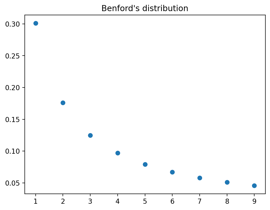
# plot distribution
plt.plot(range(1,10), Benford_pmf, 'o')
plt.title('Benford\'s distribution')
plt.show()

_images/b580409cb3f1ec64b1adb6063a57980229ff77aba943be4bd43f1563571ff400.png

Now let’s turn to some continuous random variables.

9.5. Univariate Gaussian distribution#

We write

X \sim N (μ, σ^{2})

to indicate the probability distribution

f (x | u, σ^{2}) = \frac{1}{\sqrt{2 π σ^{2}}} e^{[- \frac{1}{2 σ^{2}} (x - u)^{2}]}

In the below example, we set $μ = 0, σ = 0.1$ .

# specify parameters
μ, σ = 0, 0.1

# specify number of draws
n = 1_000_000

# draw observations from the distribution
x = np.random.normal(μ, σ, n)

# compute sample mean and variance
μ_hat = np.mean(x)
σ_hat = np.std(x)

print("The sample mean is: ", μ_hat)
print("The sample standard deviation is: ", σ_hat)

The sample mean is:  -2.8548065661503377e-05
The sample standard deviation is:  0.09990243468371045

# compare
print(μ-μ_hat < 1e-3)
print(σ-σ_hat < 1e-3)

True
True

9.6. Uniform Distribution#

\begin{array}{r} \begin{aligned} X & \sim U [a, b] \\ f (x) & = {\begin{cases} \frac{1}{b - a}, & a \leq x \leq b \\ 0, & otherwise \end{cases} \end{aligned} \end{array}

The population mean and variance are

\begin{array}{r} \begin{aligned} E (X) & = \frac{a + b}{2} \\ V (X) & = \frac{(b - a)^{2}}{12} \end{aligned} \end{array}

# specify parameters
a, b = 10, 20

# specify number of draws
n = 1_000_000

# draw observations from the distribution
x = a + (b-a)*np.random.rand(n)

# compute sample mean and variance
μ_hat = np.mean(x)
σ2_hat = np.var(x)

print("The sample mean is: ", μ_hat, "\nThe sample variance is: ", σ2_hat)
print("\nThe population mean is: ", (a+b)/2)
print("The population variance is: ", (b-a)**2/12)

The sample mean is:  15.00250459918252 
The sample variance is:  8.342970489200585

The population mean is:  15.0
The population variance is:  8.333333333333334

9.7. A Mixed Discrete-Continuous Distribution#

We’ll motivate this example with a little story.

Suppose that to apply for a job you take an interview and either pass or fail it.

You have $5 %$ chance to pass an interview and you know your salary will uniformly distributed in the interval 300~400 a day only if you pass.

We can describe your daily salary as a discrete-continuous variable with the following probabilities:

P (X = 0) = 0.95

P (300 \leq X \leq 400) = \int_{300}^{400} f (x) d x = 0.05

f (x) = 0.0005

Let’s start by generating a random sample and computing sample moments.

x = np.random.rand(1_000_000)
# x[x > 0.95] = 100*x[x > 0.95]+300
x[x > 0.95] = 100*np.random.rand(len(x[x > 0.95]))+300
x[x <= 0.95] = 0

μ_hat = np.mean(x)
σ2_hat = np.var(x)

print("The sample mean is: ", μ_hat, "\nThe sample variance is: ", σ2_hat)

The sample mean is:  17.536613589301137 
The sample variance is:  5874.314525073605

The analytical mean and variance can be computed:

\begin{array}{r} \begin{aligned} μ & = \int_{300}^{400} x f (x) d x \\ = 0.0005 \int_{300}^{400} x d x \\ = 0.0005 \times \frac{1}{2} x^{2} |_{300}^{400} \end{aligned} \end{array}

\begin{array}{r} \begin{aligned} σ^{2} & = 0.95 \times (0 - 17.5)^{2} + \int_{300}^{400} (x - 17.5)^{2} f (x) d x \\ = 0.95 \times {17.5}^{2} + 0.0005 \int_{300}^{400} (x - 17.5)^{2} d x \\ = 0.95 \times {17.5}^{2} + 0.0005 \times \frac{1}{3} (x - 17.5)^{3} |_{300}^{400} \end{aligned} \end{array}

mean = 0.0005*0.5*(400**2 - 300**2)
var = 0.95*17.5**2+0.0005/3*((400-17.5)**3-(300-17.5)**3)
print("mean: ", mean)
print("variance: ", var)

mean:  17.5
variance:  5860.416666666666

9.8. Drawing a Random Number from a Particular Distribution#

Suppose we have at our disposal a pseudo random number that draws a uniform random variable, i.e., one with probability distribution

Prob {\tilde{X} = i} = \frac{1}{I}, i = 0, \dots, I - 1

How can we transform $\tilde{X}$ to get a random variable $X$ for which $Prob {X = i} = f_{i}, i = 0, \dots, I - 1$ , where $f_{i}$ is an arbitary discrete probability distribution on $i = 0, 1, \dots, I - 1$ ?

The key tool is the inverse of a cumulative distribution function (CDF).

Observe that the CDF of a distribution is monotone and non-decreasing, taking values between $0$ and $1$ .

We can draw a sample of a random variable $X$ with a known CDF as follows:

draw a random variable $u$ from a uniform distribution on $[0, 1]$
pass the sample value of $u$ into the “inverse” target CDF for $X$
$X$ has the target CDF

Thus, knowing the “inverse” CDF of a distribution is enough to simulate from this distribution.

Note

The “inverse” CDF needs to exist for this method to work.

The inverse CDF is

F^{- 1} (u) \equiv inf {x \in R : F (x) \geq u} (0 < u < 1)

Here we use infimum because a CDF is a non-decreasing and right-continuous function.

Thus, suppose that

$U$ is a uniform random variable $U \in [0, 1]$
We want to sample a random variable $X$ whose CDF is $F$ .

It turns out that if we use draw uniform random numbers $U$ and then compute $X$ from

X = F^{- 1} (U),

then $X$ is a random variable with CDF $F_{X} (x) = F (x) = Prob {X \leq x}$ .

We’ll verify this in the special case in which $F$ is continuous and bijective so that its inverse function exists and can be denoted by $F^{- 1}$ .

Note that

\begin{array}{r} \begin{aligned} F_{X} (x) & = Prob {X \leq x} \\ = Prob {F^{- 1} (U) \leq x} \\ = Prob {U \leq F (x)} \\ = F (x) \end{aligned} \end{array}

where the last equality occurs because $U$ is distributed uniformly on $[0, 1]$ while $F (x)$ is a constant given $x$ that also lies on $[0, 1]$ .

Let’s use numpy to compute some examples.

Example: A continuous geometric (exponential) distribution

Let $X$ follow a geometric distribution, with parameter $λ > 0$ .

Its density function is

f (x) = λ e^{- λ x}

Its CDF is

F (x) = \int_{0}^{\infty} λ e^{- λ x} = 1 - e^{- λ x}

Let $U$ follow a uniform distribution on $[0, 1]$ .

$X$ is a random variable such that $U = F (X)$ .

The distribution $X$ can be deduced from

\begin{array}{r} \begin{aligned} U & = F (X) = 1 - e^{- λ X} \\ ⟹ & - U = e^{- λ X} \\ ⟹ & \log (1 - U) = - λ X \\ ⟹ & X = \frac{(1 - U)}{- λ} \end{aligned} \end{array}

Let’s draw $u$ from $U [0, 1]$ and calculate $x = \frac{l o g (1 - U)}{- λ}$ .

We’ll check whether $X$ seems to follow a continuous geometric (exponential) distribution.

Let’s check with numpy.

n, λ = 1_000_000, 0.3

# draw uniform numbers
u = np.random.rand(n)

# transform
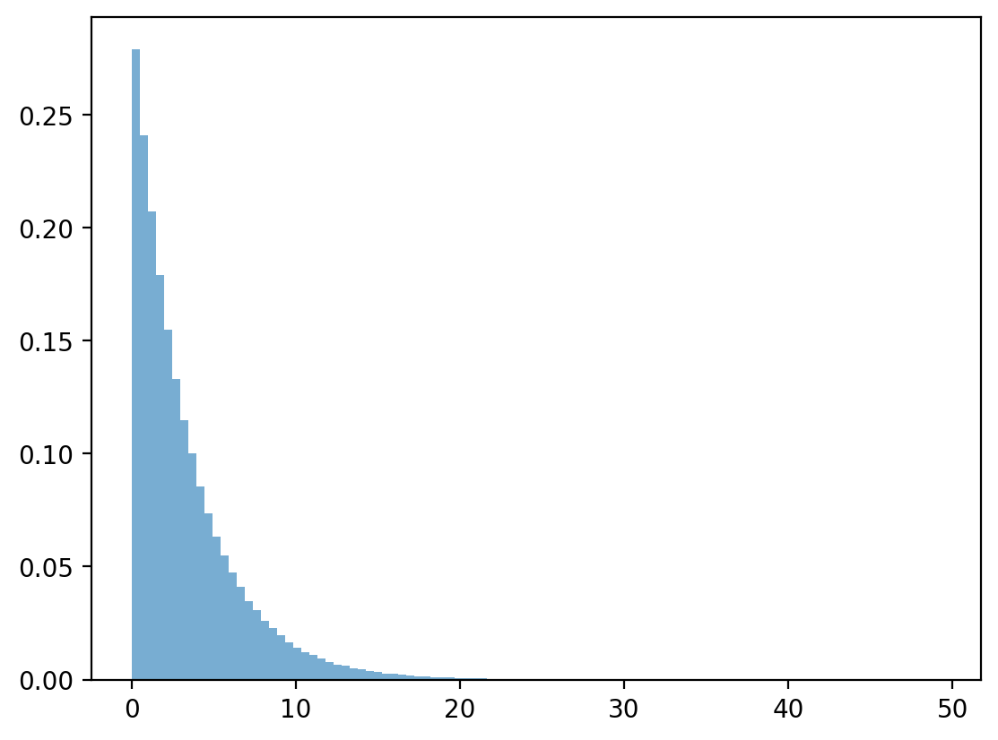
x = -np.log(1-u)/λ

# draw geometric distributions
x_g = np.random.exponential(1 / λ, n)

# plot and compare
plt.hist(x, bins=100, density=True)
plt.show()

_images/944346de0ed7bceee36224a4f04876d9e1a922f353e56741054a31c8f9f6ad89.png

plt.hist(x_g, bins=100, density=True, alpha=0.6)
plt.show()

_images/0bf4299ae52fd659014f4440a47f37e64429b834b167ad41260b348eb0965f40.png

Geometric distribution

Let $X$ distributed geometrically, that is

\begin{array}{r} \begin{aligned} Prob (X = i) & = (1 - λ) λ^{i}, λ \in (0, 1), i = 0, 1, \dots \\ \sum_{i = 0}^{\infty} Prob (X = i) = 1 ⟷ (1 - λ) \sum_{i = 0}^{\infty} λ^{i} = \frac{1 - λ}{1 - λ} = 1 \end{aligned} \end{array}

Its CDF is given by

\begin{array}{r} \begin{aligned} Prob (X \leq i) & = (1 - λ) \sum_{j = 0}^{i} λ^{i} \\ = (1 - λ) [\frac{1 - λ^{i + 1}}{1 - λ}] \\ = 1 - λ^{i + 1} \\ = F (X) = F_{i} \end{aligned} \end{array}

Again, let $\tilde{U}$ follow a uniform distribution and we want to find $X$ such that $F (X) = \tilde{U}$ .

Let’s deduce the distribution of $X$ from

\begin{array}{r} \begin{aligned} \tilde{U} & = F (X) = 1 - λ^{x + 1} \\ 1 - \tilde{U} & = λ^{x + 1} \\ \log (1 - \tilde{U}) & = (x + 1) \log λ \\ \frac{\log (1 - \tilde{U})}{\log λ} & = x + 1 \\ \frac{\log (1 - \tilde{U})}{\log λ} - 1 & = x \end{aligned} \end{array}

However, $\tilde{U} = F^{- 1} (X)$ may not be an integer for any $x \geq 0$ .

So let

x = ⌈ \frac{\log (1 - \tilde{U})}{\log λ} - 1 ⌉

where $⌈ . ⌉$ is the ceiling function.

Thus $x$ is the smallest integer such that the discrete geometric CDF is greater than or equal to $\tilde{U}$ .

We can verify that $x$ is indeed geometrically distributed by the following numpy program.

Note

The exponential distribution is the continuous analog of geometric distribution.

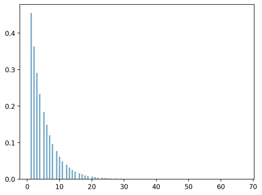
n, λ = 1_000_000, 0.8

# draw uniform numbers
u = np.random.rand(n)

# transform
x = np.ceil(np.log(1-u)/np.log(λ) - 1)

# draw geometric distributions
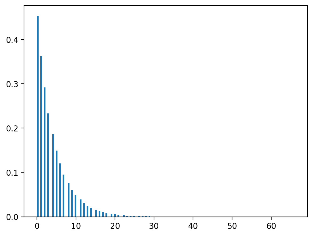
x_g = np.random.geometric(1-λ, n)

# plot and compare
plt.hist(x, bins=150, density=True)
plt.show()

_images/42f7033084cfb5772f21bd9f4816ee69a4d18cc8cc9164a9dfd260c73d6498eb.png

np.random.geometric(1-λ, n).max()

np.int64(74)

np.log(0.4)/np.log(0.3)

np.float64(0.7610560044063083)

plt.hist(x_g, bins=150, density=True, alpha=0.6)
plt.show()

_images/650e5b776e8522db8f9ca2d66eac5e29d665918522e9c9771388bcfaad9d5d5b.png